| OBJECTID | GlobalID | type | source | poly_DateCurrent | mission | incident_name | incident_number | area_acres | description | FireDiscoveryDate | CreationDate | EditDate | displayStatus | geometry | |
|---|---|---|---|---|---|---|---|---|---|---|---|---|---|---|---|
| 0 | 3025 | 04ba1d01-c043-478f-ad62-e7eeb903cf09 | Heat Perimeter | FIRIS | 2025-01-01 05:39:02.359000+00:00 | CA-SBC-OAK-N40Y | Oak | None | 41.998143 | FIRIS Perimeter | NaT | 2025-01-01 05:37:18+00:00 | NaT | Inactive | POLYGON ((-120.24304 34.88387, -120.24302 34.8... |
| 1 | 3026 | 4551a5e4-e94d-46e2-9aac-73cc4314c946 | Heat Perimeter | FIRIS | 2025-01-02 05:16:55.340000+00:00 | CA-SDU-BORDER1-N40Y | None | None | 16.911501 | FIRIS Perimeter | NaT | 2025-01-02 05:13:35+00:00 | NaT | Inactive | MULTIPOLYGON (((-116.82928 32.59686, -116.8293... |
| 2 | 3027 | 2b1329f3-5b39-4c0e-ad34-1250e436e0e1 | Heat Perimeter | FIRIS | 2025-01-07 22:11:19.142000+00:00 | CA-LFD-PALISADES-N57B | None | None | 771.572356 | FIRIS Perimeter | NaT | 2025-01-07 22:09:29+00:00 | NaT | Inactive | MULTIPOLYGON (((-118.55013 34.06195, -118.5501... |
| 3 | 3028 | a766c1b5-1d8e-43b3-9aac-02358de18d35 | Heat Perimeter | FIRIS | 2025-01-07 23:17:35.698000+00:00 | CA-LFD-PALISADES-N57B | None | None | 1261.520779 | FIRIS Perimeter | NaT | 2025-01-07 23:13:25+00:00 | NaT | Inactive | MULTIPOLYGON (((-118.55013 34.06195, -118.5501... |
| 4 | 3029 | 72049d43-03fe-4cc1-899a-fe2eb43934e7 | Heat Perimeter | FIRIS | 2025-01-07 23:17:39.454000+00:00 | CA-LFD-PALISADES-N57B | None | None | 1261.520779 | FIRIS Perimeter | NaT | 2025-01-07 23:13:25+00:00 | NaT | Inactive | MULTIPOLYGON (((-118.55013 34.06195, -118.5501... |
NR 218
What is a computer
A machine that manipulates data following a list of programmed instructions
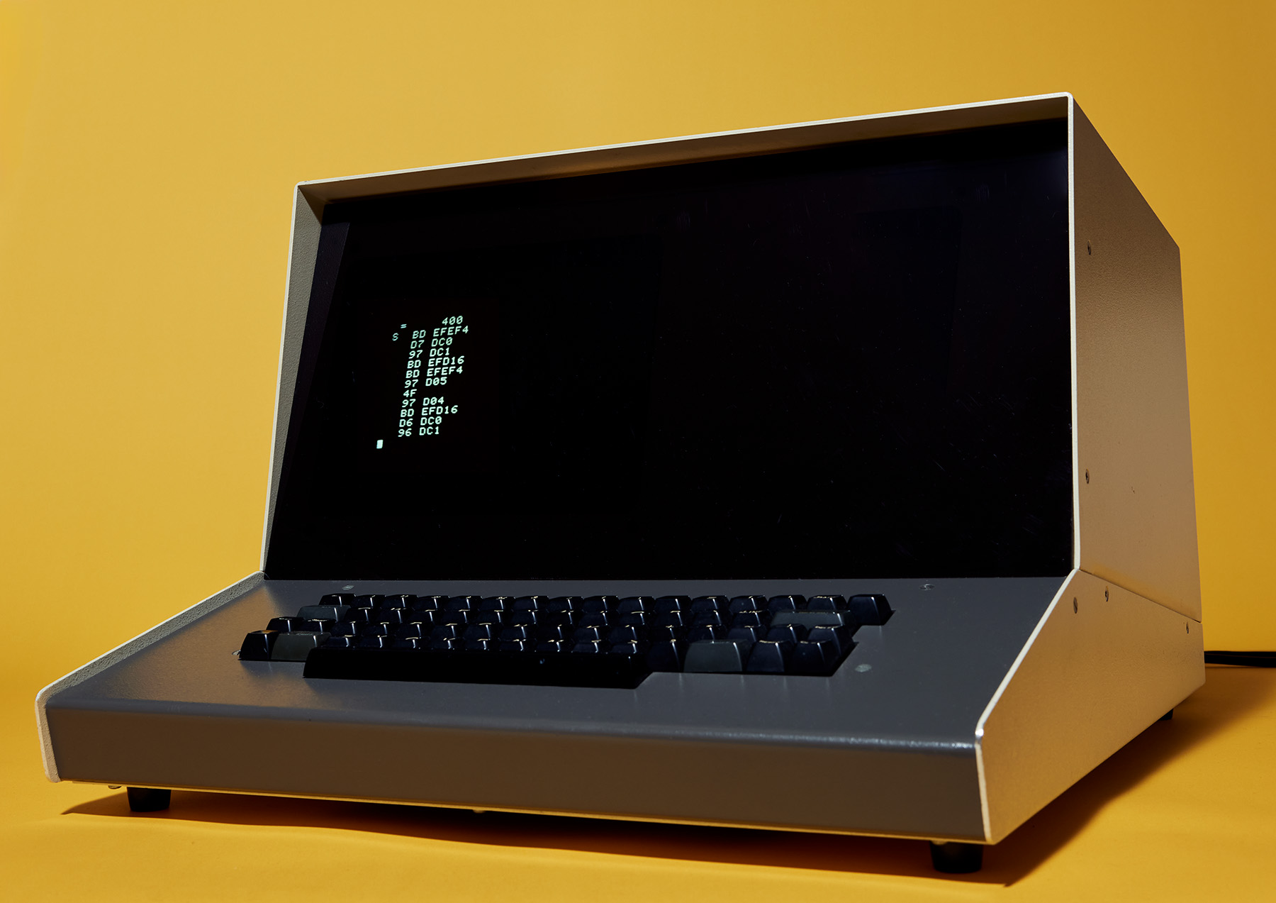
Image Source: Wikimedia commons
Data
- “Related items of (chiefly numerical) information considered collectively, typically obtained by scientific work and used for reference, analysis, or calculation.”
- “Quantities, characters, or symbols on which operations are performed by a computer, considered collectively. Also (in non-technical contexts): information in digital form.” -OED
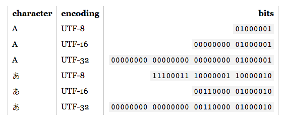
- Data is stored on a computer as zeros and ones .
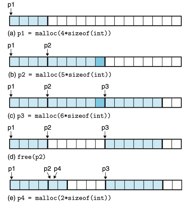
- Data is stored at some physical location on the disk, and a pointer is saved which is later used to find the file.
- The details of this are managed for you by applications or programming languages by representing this relationship as a path.

Image Source: Wikimedia /Sven
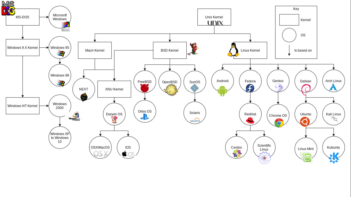
Family tree of modern general purpose operating systems. With the exception of Windows (which derives from MS-DOS) all widely used modern general purpose OSs are based on UNIX.
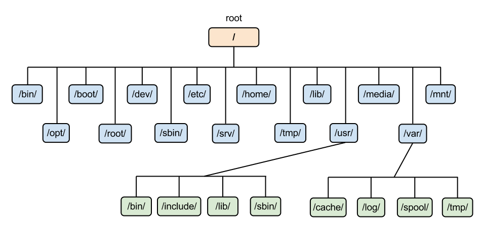
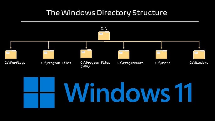
File Paths and Directories
Data Storage
- We store data in computer-readable format in files
- Sometimes files store data as text (often called human readable files)
- Other times there are just 1s and 0s (binary file)
- Even the human readable files are ultimately stored as 1s and 0s (more on that)
File Paths and Directories
File Organization and Computer Hygiene
Be kind to your future self - keep your files organized:
- Use directories (a.k.a folders)
- Use descriptive names:
- e.g.
slo_county_26910.geojsonnotcounty.geojson
- e.g.
- Don’t put spaces in file or directory names (see this)
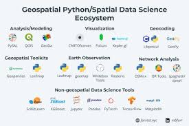
What is GIS?
Computer-based tools used to store, visualize, analyze, and interpret geographic data
OR
Collection of computer hardware, software, data, personnel, and work procedures to store, update, manipulate, analyze, and display all forms of geographic information.
![]()
![]()
![]()
Why use GIS
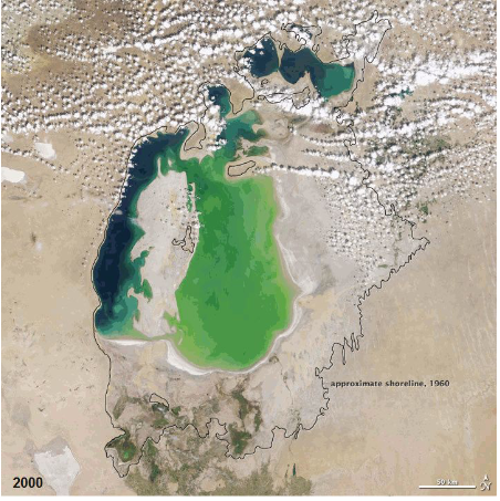
Monitor and understand our planet
Planning
Disaster Response
Software
- This class will be taught using QGIS.
- Software changes - We will focus on building an understanding of the concepts that will allow you to successfully use any GIS software.
- I might show examples of analysis using other tools, particularly Python.
There are many other common (GUI based) GIS software platforms:
- ESRI (ArcGIS suite)
- GRASS
- Google Earth Engine
- Google Earth Pro
- ENVI
- SAGA
- etc…
There are also command line tools
- GDAL
- PDAL
- WhiteBox Tools
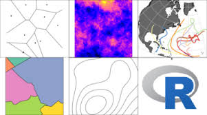
Additionally, GIS can be performed using scripting languages
- Python
- R
- Javascript
- Julia
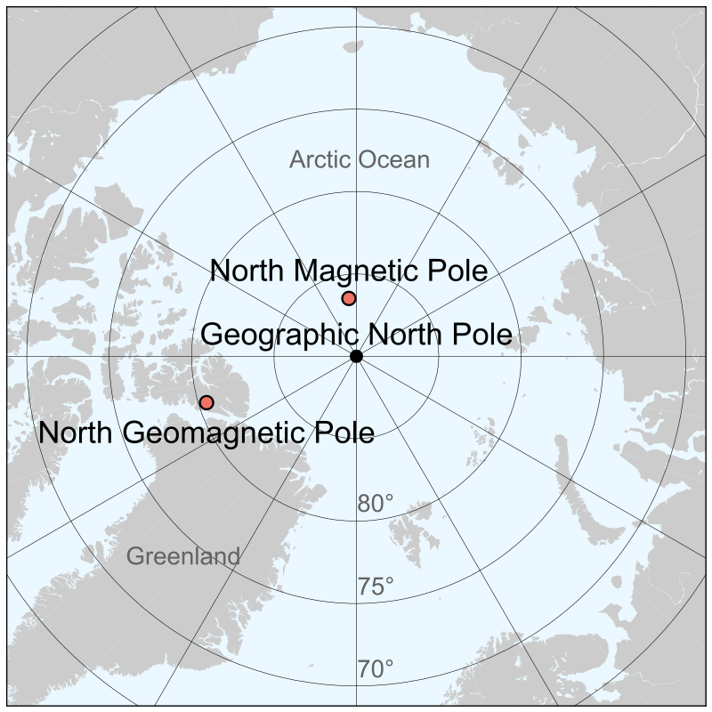
- btw, currently North is South!
- Magnetic and Geomagnetic poles?
Layers
Models representing different aspects of the physical world 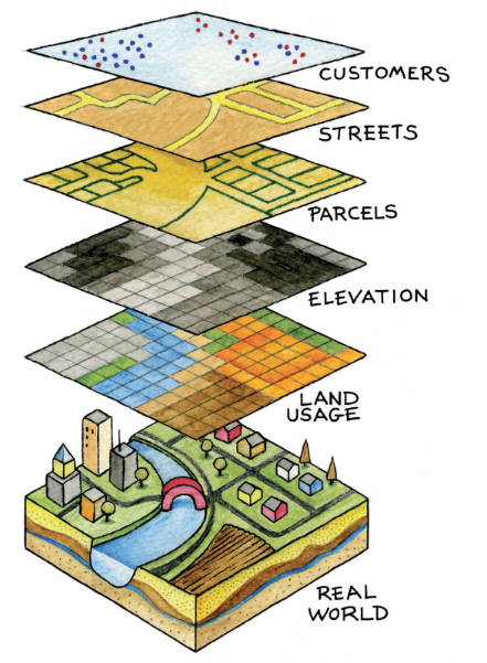
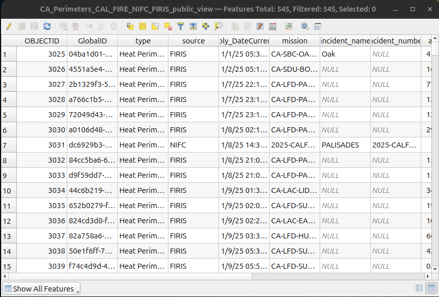
Right-click layer –> Open Attribute Table
Map Types
There are a few types of maps:
Mental Maps
- Psychological tools that we all use every day.
- Stored in our brain
- To get from one place to another, or to understand and situate events that we hear about
- Reflect the amount and extent of geographic knowledge and spatial awareness that we possess
Using a blank sheet of paper, take five minutes to draw a map from memory of San Luis Obispo
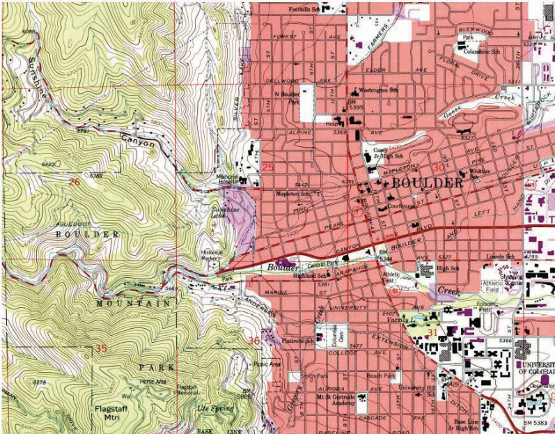
Reference - shows location information, often represent geographic reality accurately, topographic maps for example
Reference - shows location information, often represent geographic reality accurately…
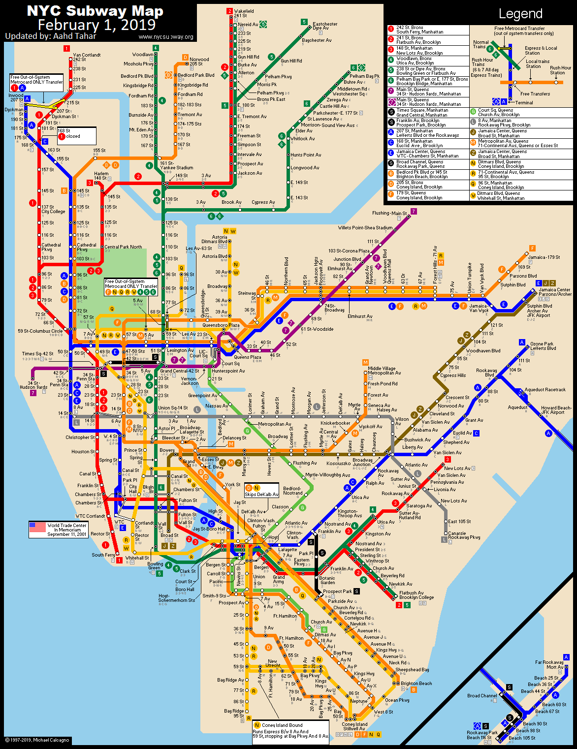
But not always. A subway map is also a reference map. It represents topological relationships accurately in a schematic way for ease of navigation
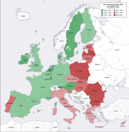
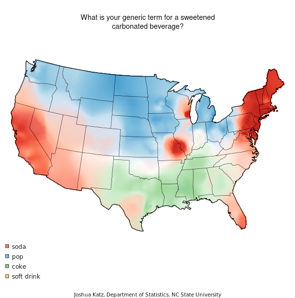
Thematic - shows how one or more factors are distributed across space, such as a map of malaria infection rates
Dynamic / Interactive
- maps that change depending on user input
Show code
from pathlib import Path

import folium
import geopandas as gpd

aoi_path = Path('assets/Eaton_Perimeter_20250121.geojson')
aoi = gpd.read_file(aoi_path)

# grab centroids
c = aoi.to_crs(epsg=26910).dissolve().centroid.to_crs(epsg=4326).item()

# map
map = folium.Map(
  location=[c.y, c.x],
  tiles='OpenStreetMap',
  zoom_start=12
)

# perimeter
geo_j = folium.GeoJson(data=aoi.__geo_interface__,
  style_function=lambda feature: {
    'color': 'red',
    'weight': 2,
    'fill': False,
    },
    name='Fire Perimeter'
  ).add_to(map)
# layer control

map
Make this Notebook Trusted to load map: File -> Trust Notebook
:::
Map Conventions
Mapping conventions facilitate effective conveyance of information. In most cases using them is a good idea (but not necessarily always)

The Blue Marble photograph in its original orientation.
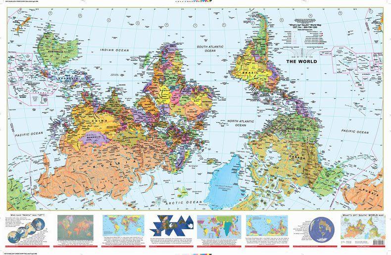
South’s up!
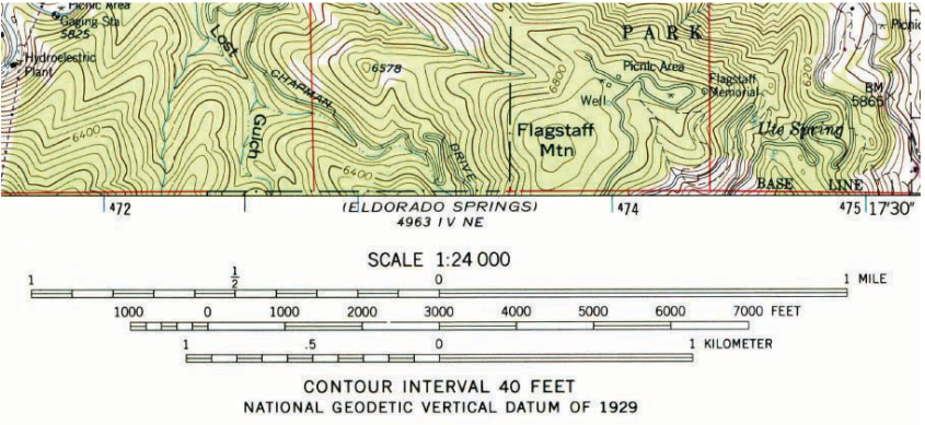
Map Scale
The factor of reduction of the world so it fits on a map
- You need to shrink things to make a map
- On reference maps it is generally important to include a scale bar
![]()
- Representative fraction (RF) describes scale as a simple ratio
- The numerator, which is always unity (i.e., 1), denotes map distance.
The denominator denotes ground or “real-world” distance. - unit neutral
- Large vs small, 1:1,000 > 1:1,000,000
- Large shows more detail
- The numerator, which is always unity (i.e., 1), denotes map distance.
Map Scale
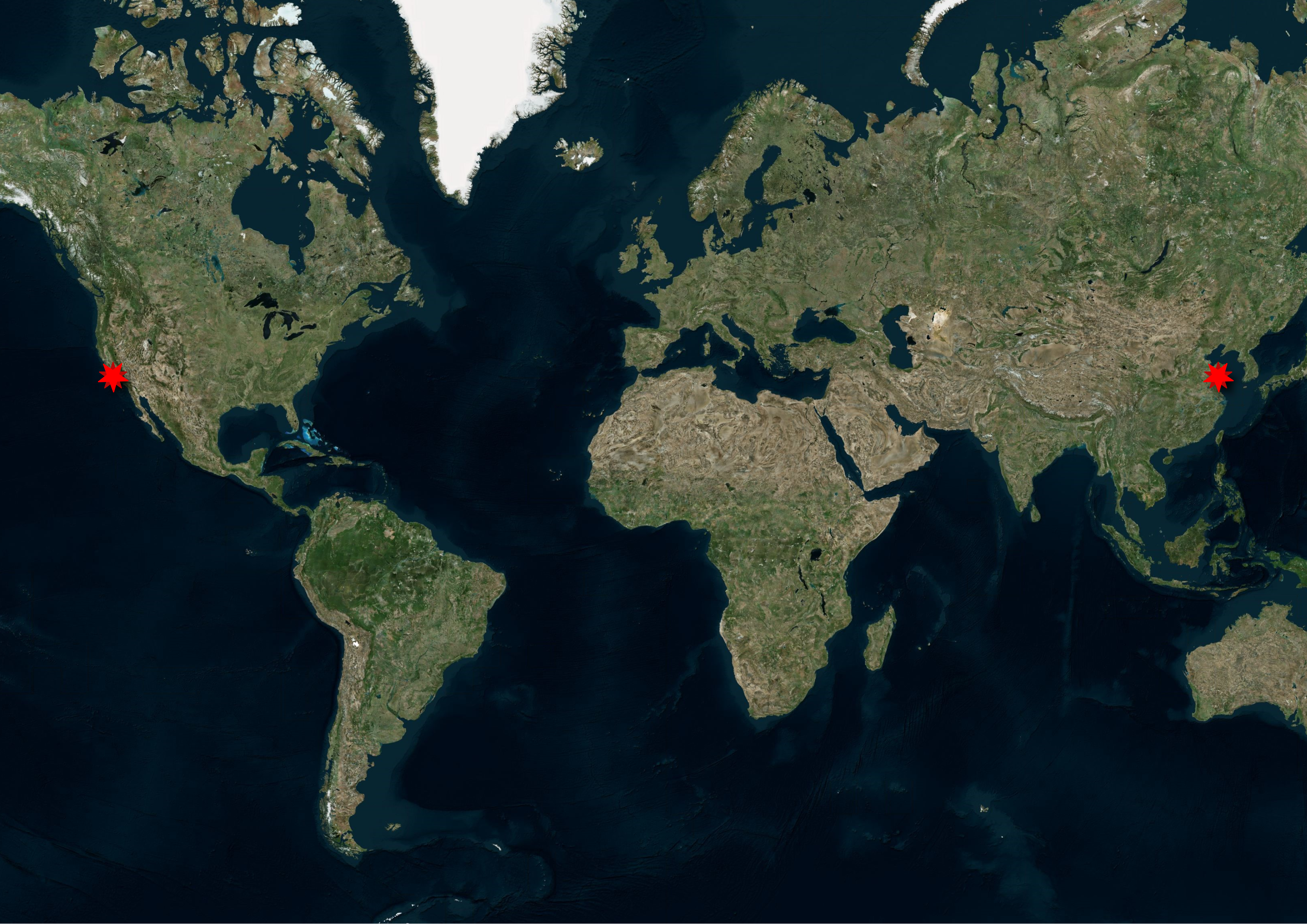
DMS to DD conversion
128° 40’ 52.0428” W
128° 40’ 52.0428” W
128° 40’ 52.0428” W
128° 40’ 52.0428” W
128° 40’ 52.0428” W
128
128 + (40 / 60)
128 + (40 / 60) + ( 52.0428 / 60\(^{2}\) )
-128.68112299
The negative is important! SLO vs. off the coast of Shandong
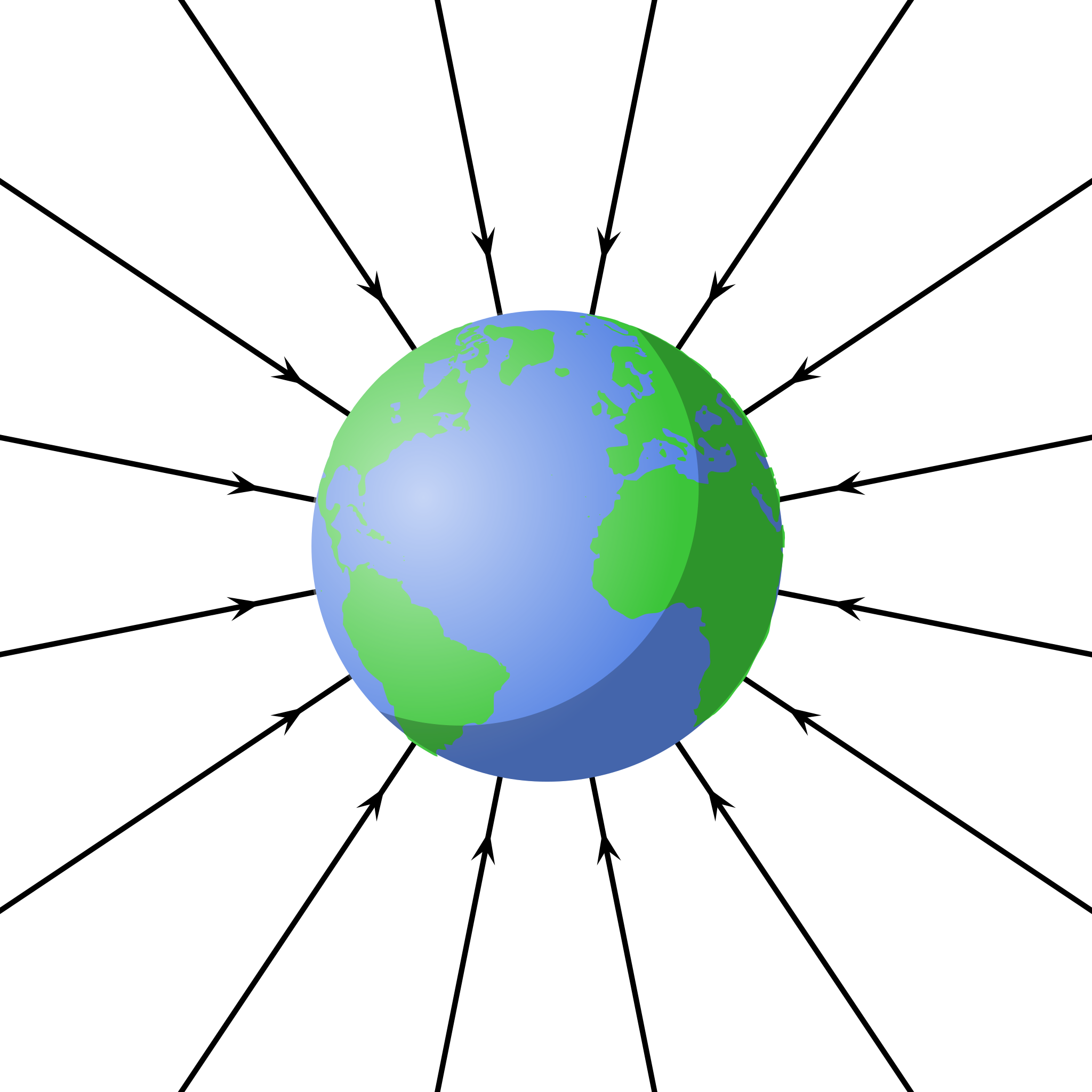
Spheroids and Geoids
A geoid is an approximation of the true shape of the earth
\(\circ\) As defined by its gravitational field rather than its topography 1
\(\circ\) Gravitational field found by finding equipotential surfaces
\(\circ\) The geoid is the specific equipotential surface that best approximates mean sea level (MSL) on a global basis
\(\circ\) MSL diverges from the geoid by up to 2 m in places.
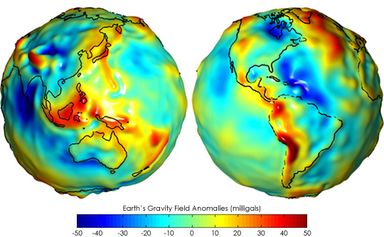
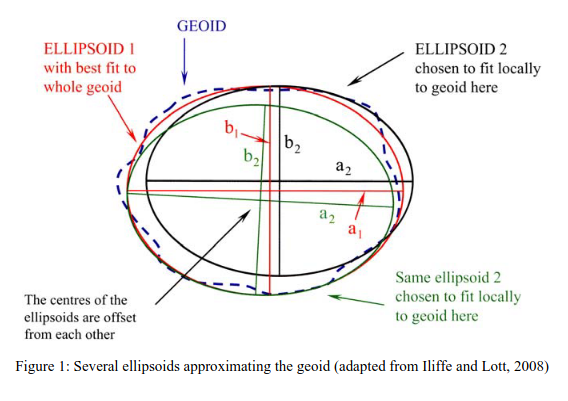
Spheroids and Geoids
The geoid is pretty complex…
so the surface is approximated using a spheroid (also called an ellipsoid of revolution)
A GCS is based on a reference model of the Earth, usually a sphere or spheroid (ellipsoid)

Datums
- A datum is a spheroid with an origen point and orientation aligning it for a particular use.
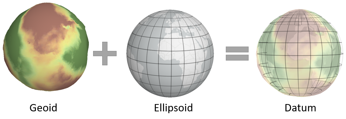
Image Source: Manny Gimond
- A local datum matches a geoid to an ellipsoid to fit a local context, e.g.
- NAD27 (North American Datum of 1927) is widely used in the U.S., especially in older maps.
- ED50 (European Datum of 1950) is common in Western Europe.

Image Source: Manny Gimond
- A geocentric datum aligns the centroid of the geoid to the center of the ellipsoid

Image Source: Manny Gimond
- Common datums used in North America
| Datum | Type | Typical use in North America |
|---|---|---|
| NAD27 | Local | Legacy U.S., Mexico, and Central America maps |
| NAD83 | Regional geocentric* | Standard for most modern U.S. and Canadian mapping |
| NAD83 (2011) | Regional geocentric | High-accuracy modern U.S. realization of NAD83 |
| WGS84 | Global geocentric | GPS and global web mapping |
* NAD83 is Earth-centered in concept, but regionally realized and not identical to a fully global geocentric frame.
Projections
- Mathematical transform for transforming 3D Earth to 2D map
- i.e. project the latitude and longitude to x any coordinates on a plane
- There are infinite ways to do this, they all cause distortion
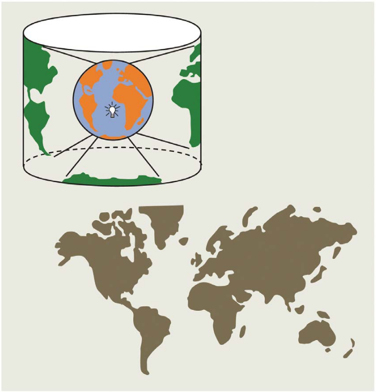
Projections
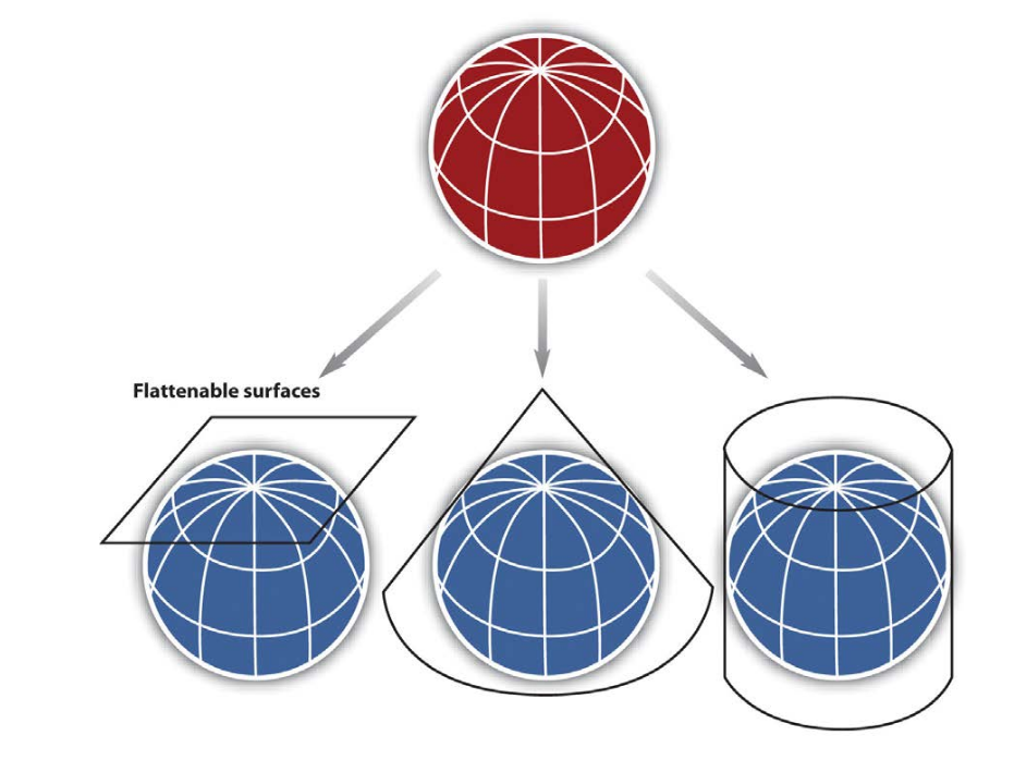
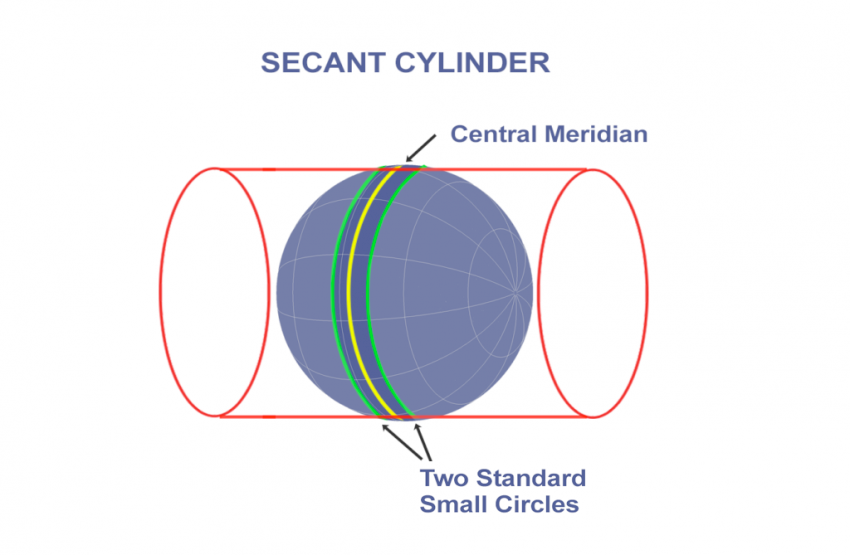
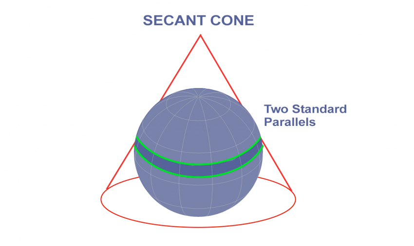
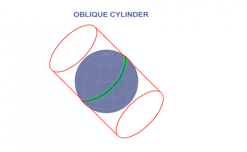
Imagine a lightbulb inside of the earth, shining out and projecting the shadows of the continents onto a developable surface (flattenable surface).
There are three commonly used developable surfaces
- plane
- cone
- cylinder
- The developable surface can be oriented in many ways.
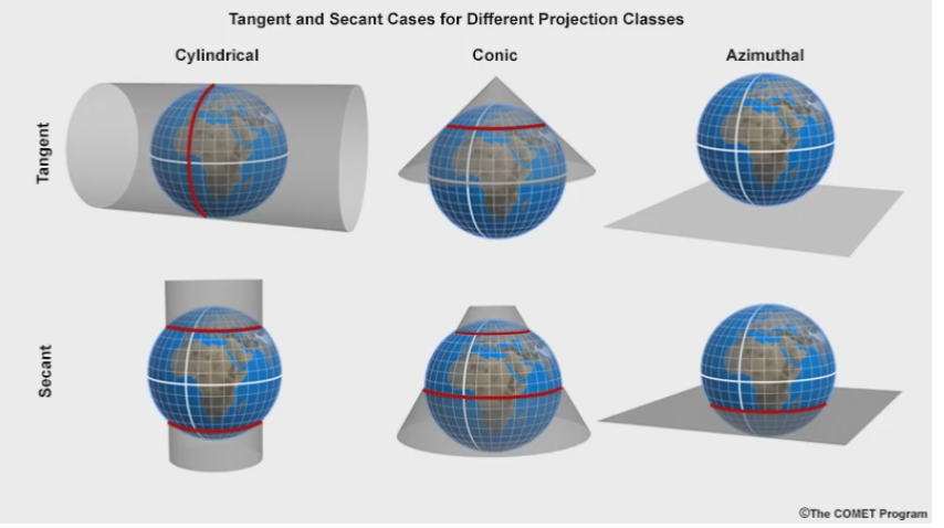
- Each developable surface can be in one of two cases tangent and secant
- The aspect of the projection is the orientation of the developable surface relative to the axis of the earth
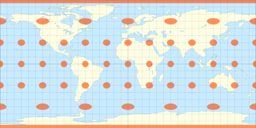
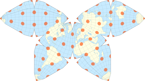
Tissot’s indicatrix
Shows linear, angular, and areal distortions of mapsEquidistant projections
- Maintains distance between points in one direction (usually north-south)
- Angles and shapes are not preserved
- Good for small-scale maps that cover large areas
- Often used for global thematic maps
Conformal map projections
- Preserve angles (also known as bearings) between locations
- Used for navigational purposes
- Areas tend to be quite distorted
- Shapes are more or less preserved over small areas, at small scales areas become wildly distorted
- e.g. Mercator projection (with normal aspect) is famous for distorting Greenland
Equal area or equivalent projections
- Preserve area
- Distort angles
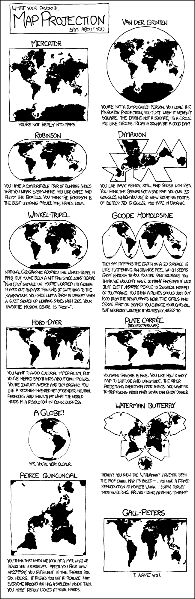
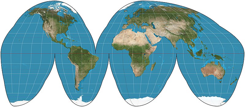
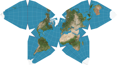
Weird projections
- Often made as compromises between types of distortion
- Like the Waterman Butterfly
![]()
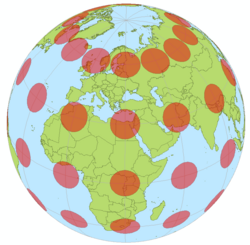
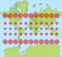 Left: circles of equal area on globe. Right: same circles on Mercator projection.
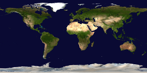
 Top: True-color satellite image of Earth in equirectangular projection.
Bottom: Equirectangular projection with Tissot’s indicatrix.
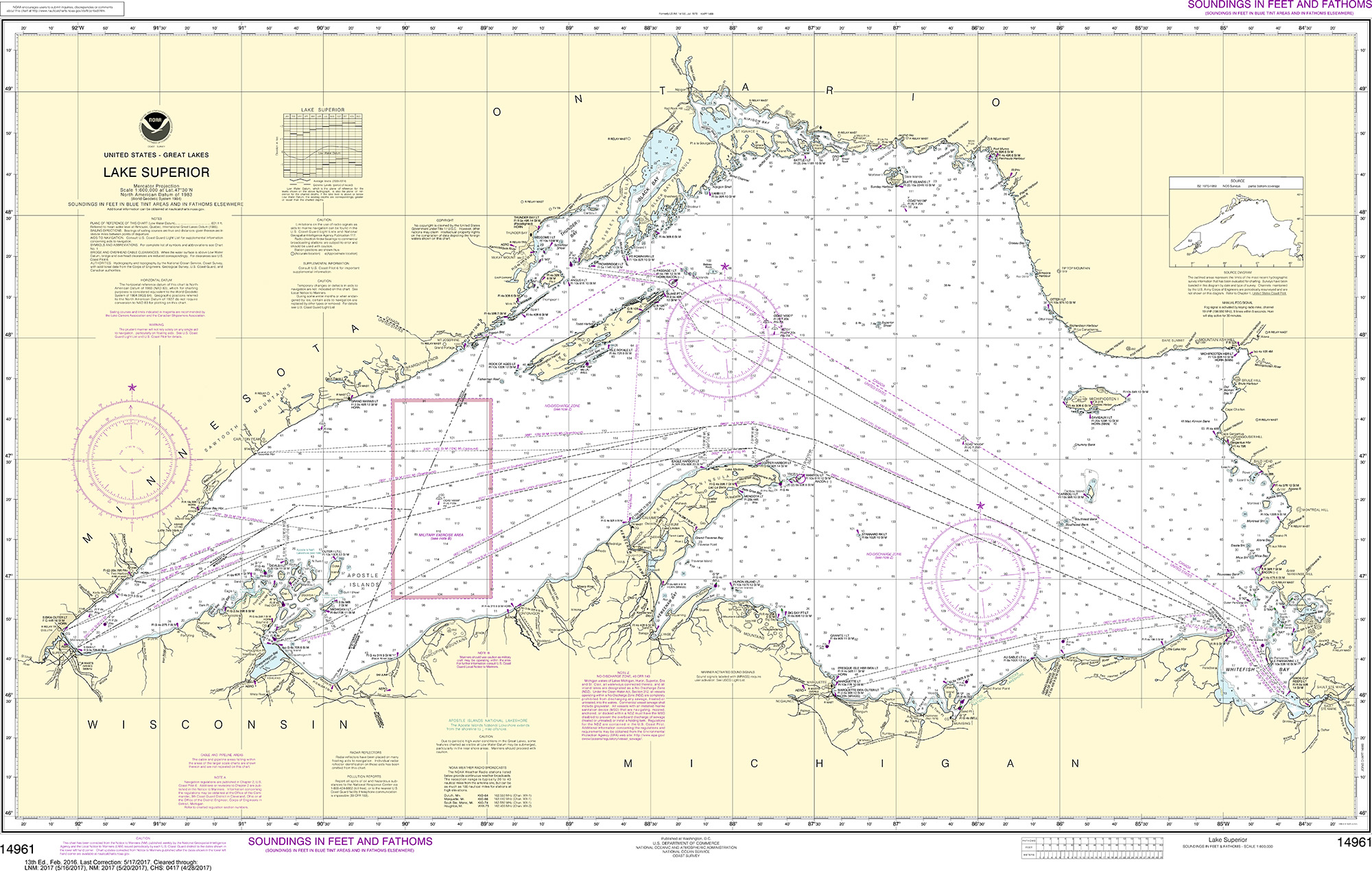
Top: Nautical Chart of Lake Superior in Mercator projection. Bottom: Mercator projection.
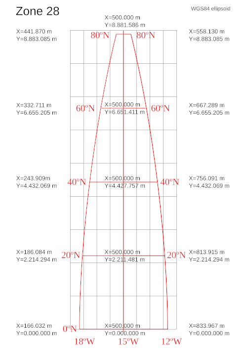
UTM
Universal Transverse Mercator (UTM)
- a projection and accompanying projected coordinate system
- Divided into 60 narrow zones
- Does not cover polar regions*
- Large north-south extent with low distortion
*Polar Stereographic is for used for conformal polar
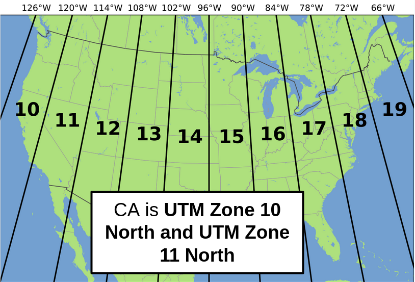
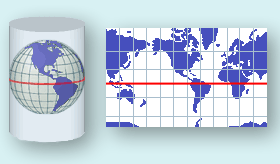
Image Source: wikimedia
- Open QGIS
- Use QuickMapServices to add a global Satellite coverage layer.
- In the drop down menus, go to Project –> Preferences then select the CRS tab on the left
- In the filter box type “26910”
- Under Predefined Coordinate Reference Systems select NAD83 / UTM zone 10N
- Click Apply and OK
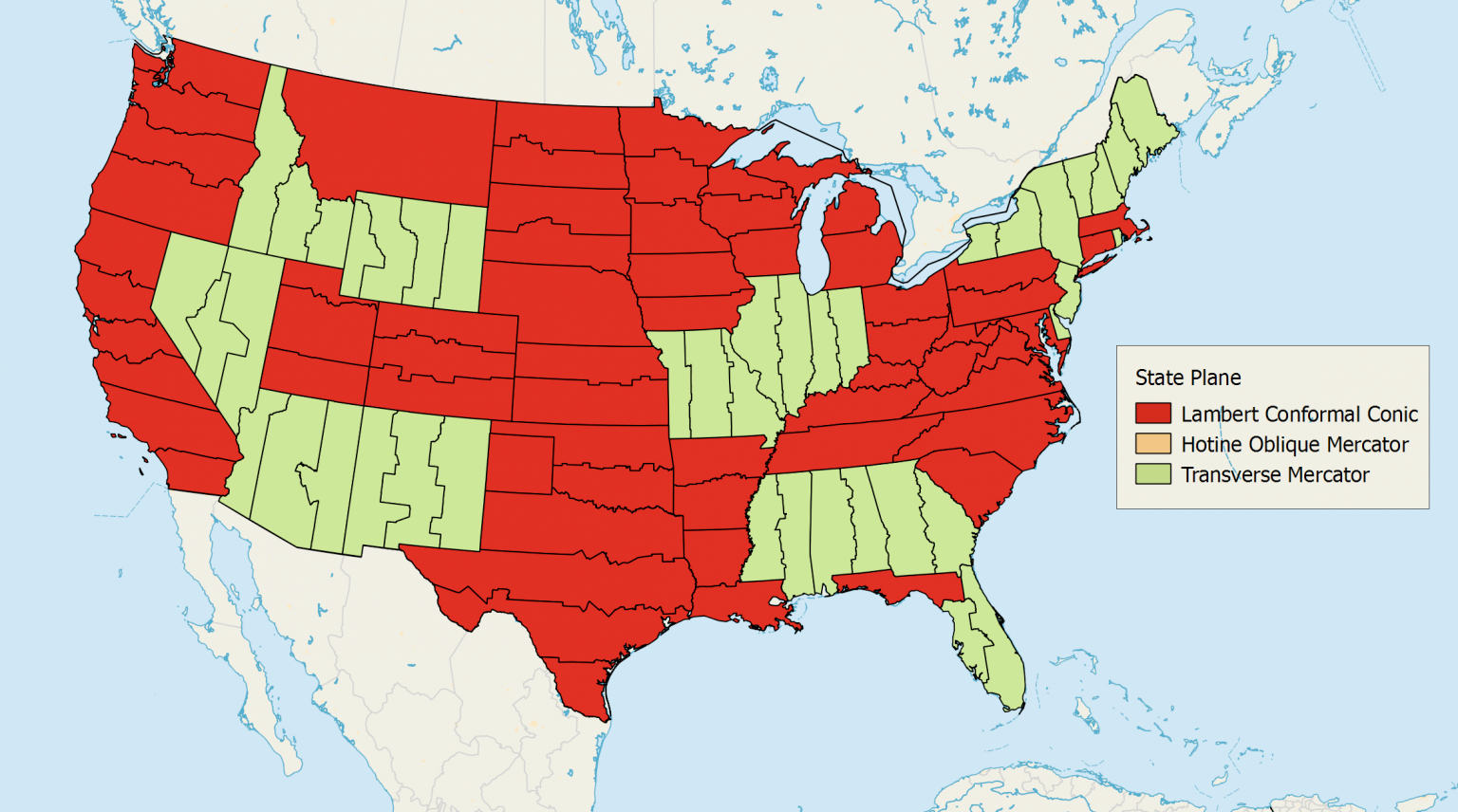
State Plan System
Each State Plane Coordinate System zone uses a map projection based on its geographic orientation.
e.g.
- Transverse Mercator Projection
- Lambert Conformal Conic Projection
- Hotine Oblique Mercator Projection
- Reproject the global satellite image from the last slide to EPSG:2227 (California zone 3)
- Scroll to zoom in on South Africa. What do you notice?
- Download
SPR_data.ziphere (right-click and “save link as”) - Extract the file (Linux, Windows, Mac), and place in appropriate file location (Remember, organize your files!)
- Open QGIS
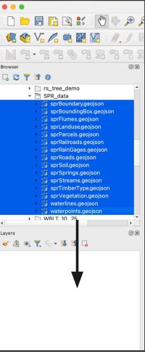
Open the files from the directory you just extracted
Method 1
- Use the file location in the ‘Browser’ panel
- Drag and and drop files into the Layers Panel
![]()
Method 2
- Press
ctrl-shift-v(cmd-shift-von Mac) - Click
![]() to browse for file then click
to browse for file then click ![]() .
.
- You can select multiple files at once when browsing
- Close window when finished.
![]()
 to browse for file then click
  .
.
Now the layers should be visible in the panel, and on the map
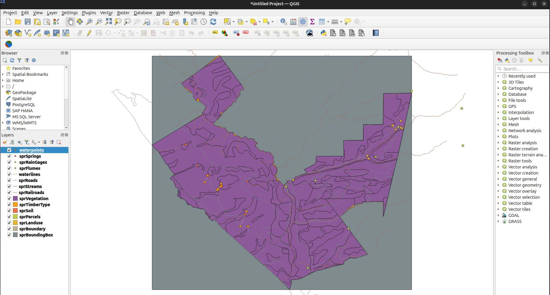
- Toggle on/off layers by clicking checkboxes
- Change layer order by dragging within panel
- What do the little icons between the check and the layer name mean?
- Right click a layer, select Open Attribute Table
- Select rows of attribute table by clicking on the left edge (where they are numbered)
- Note that the corresponding features are highlighted on the map
Panning and zooming (The mouse wheel also zooms while in pan mode)
Select tools
Info
Basemaps
- Click Plugins –> Manage and install Plugins
- Search for QuickMapServices
- Click Install Plugin
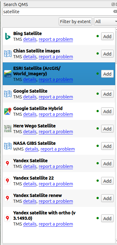
- Now on the right there should be a Search QMS bar
- Search for satellite
- Pick one (ESRI is a good choice, or Bing)
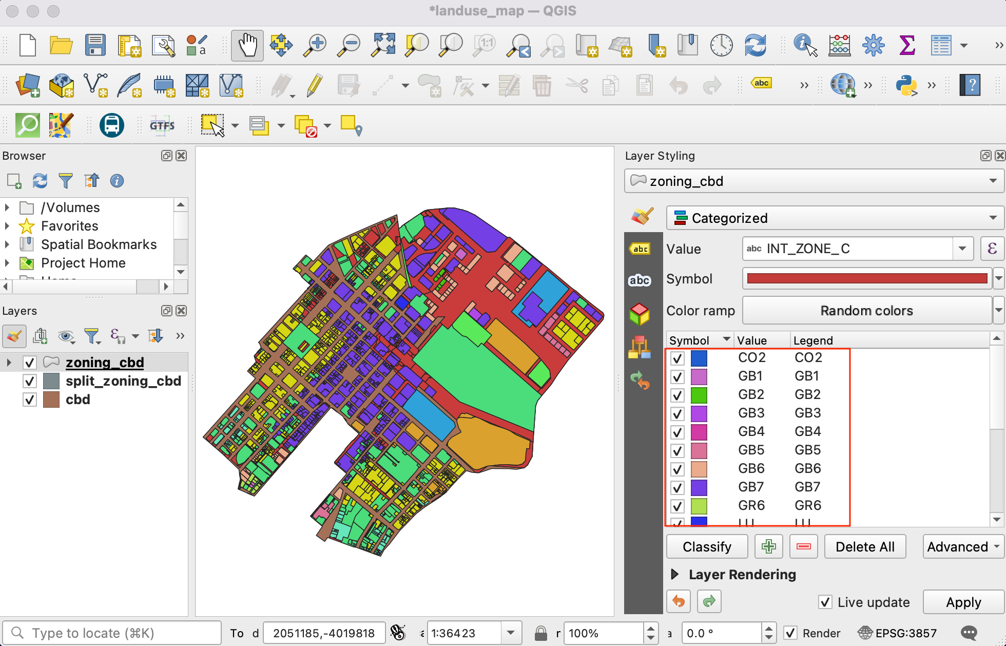
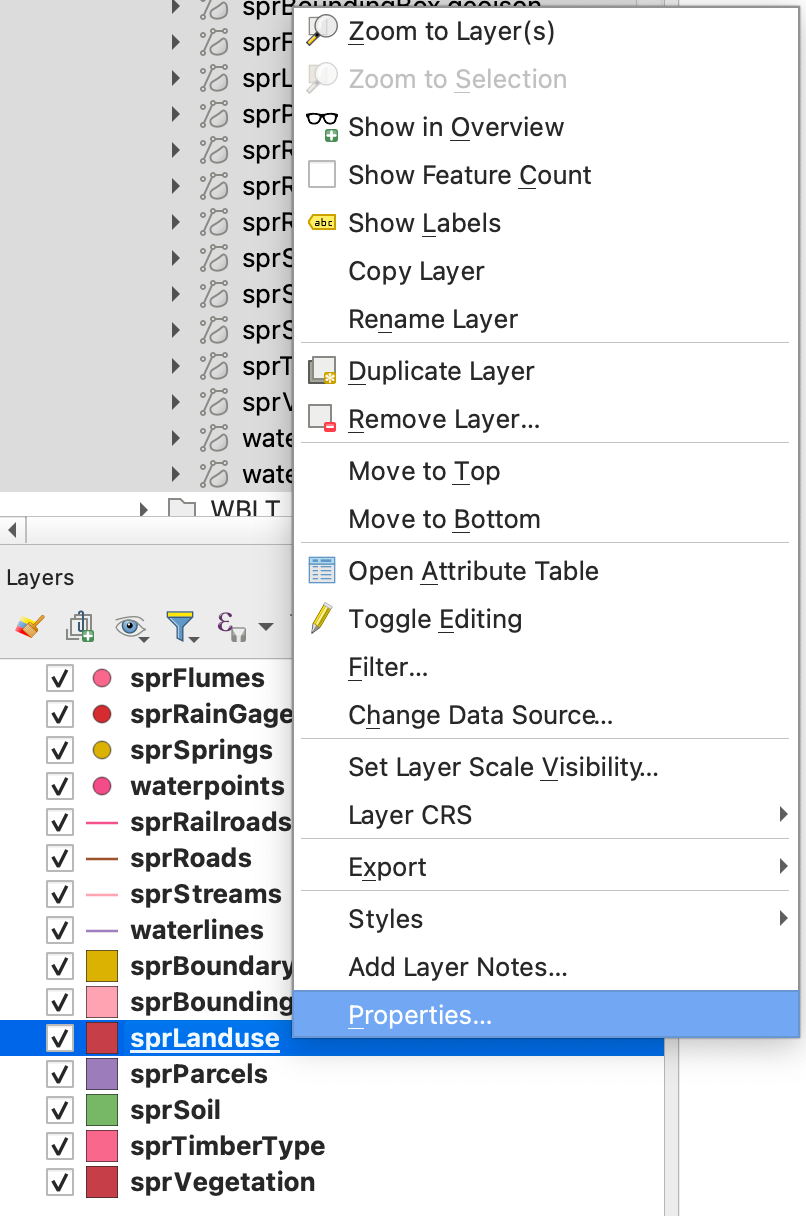
Symbology - categorized
- Right click the “sprLanduse” layer
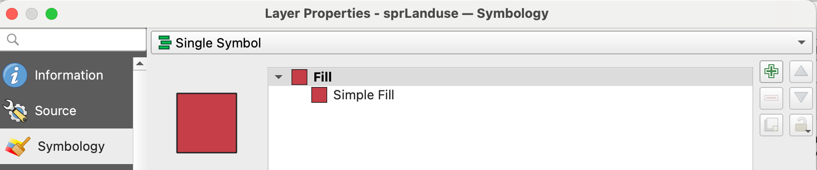
- Go to properties
- Select the symbology tab
- Go to properties
- Experiment with basic symbology
- Right click the “sprLanduse” layer
- Go to properties
- Select the symbology tab
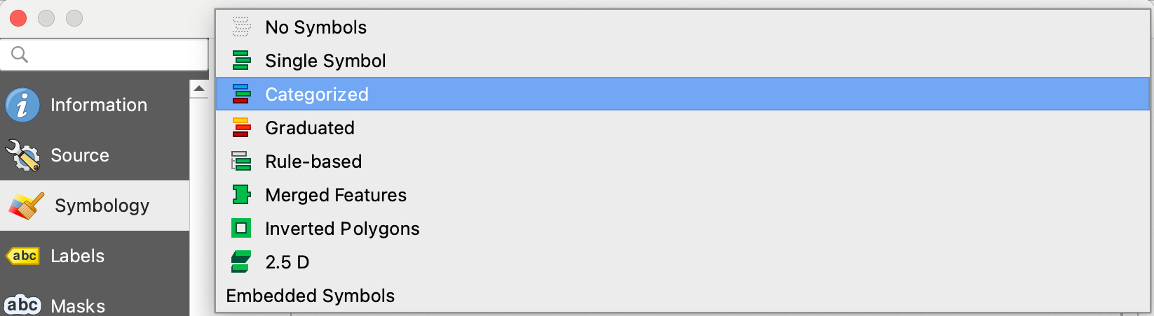
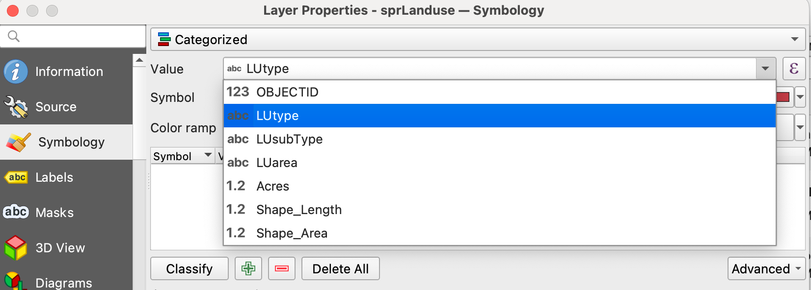
- From the dropdown menu, select “categorized”
- Select “LUtype” from the “Value” dropdown menu, and click “Classify”
- From the dropdown menu, select “categorized”
- Select the symbology tab
- Go to properties
- Right click the “sprLanduse” layer
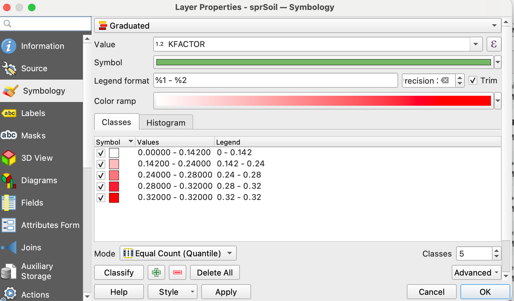
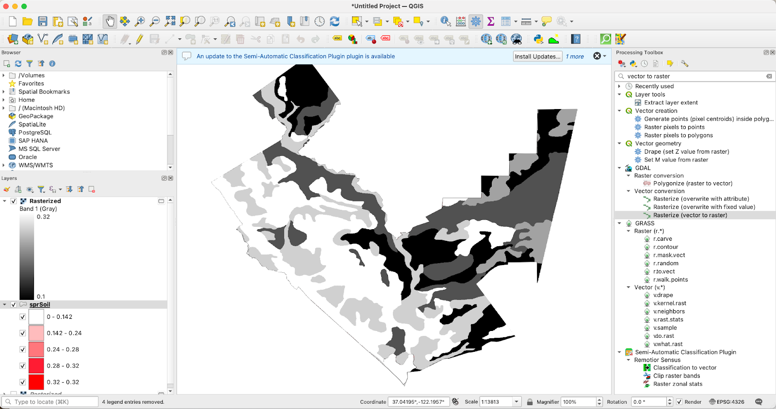
Symbology - Numerical
- Experiment with numerical symbology
- Right click the “sprSoil” layer
- go to properties
- Select the symbology tab
- From the dropdown menu, select “Graduated”
- Select “KFACTOR” from the “Value” dropdown menu
- click “Classify”, then “Apply”
- Select “KFACTOR” from the “Value” dropdown menu
- From the dropdown menu, select “Graduated”
- Select the symbology tab
- go to properties
- Right click the “sprSoil” layer
Print Layout For Maps
- Click Project > “New Print Layout”
- Give it a name and click “OK”
- Click add map (
![]() )
) - Click and drag a box onto the map canvas
to draw a box. This is where the map will
be positioned- To reposition things use move item content (
![]() )
)
- Click and drag map to pan
- Scroll with mouse wheel to change zoom (hold control for finer control)
- To reposition things use move item content (
- Click add map (
- Give it a name and click “OK”
 )
) )
)
Print Layout - Add Legend
Add a Legend:
- Click the add legend button (
![]() ), or from drop down menu Add Item > Add Legend
), or from drop down menu Add Item > Add Legend
- Draw a box to position the legend
 ), or from drop down menu Add Item > Add Legend
Edit legend items by going to Item Properties > Legend Items, and unchecking Auto Update
Buttons will appear to add or remove items 
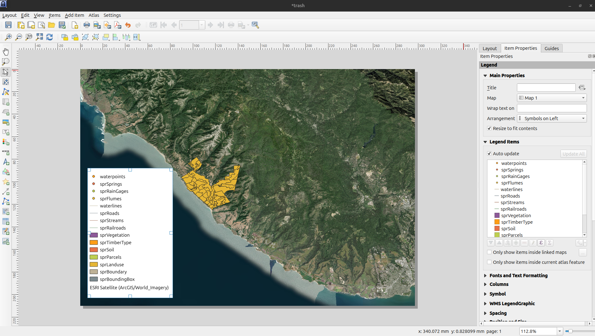
What Are some problems here
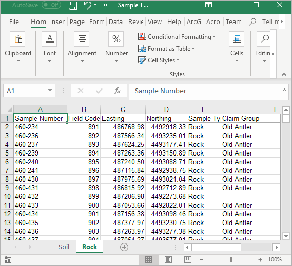
Reading a CSV with QGIS
link to file (right-click and “save link as”)
Either Layer --> Add Layer -->> Add Delimited Text Layeror press control V (command V on Mac)
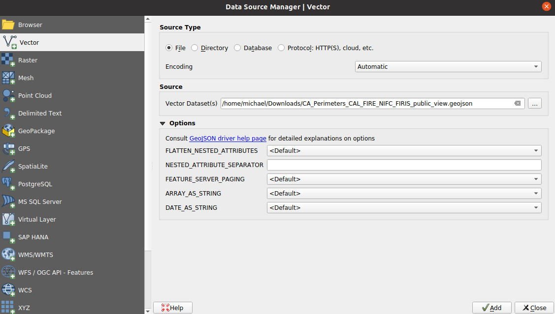
Reading a CSV with QGIS
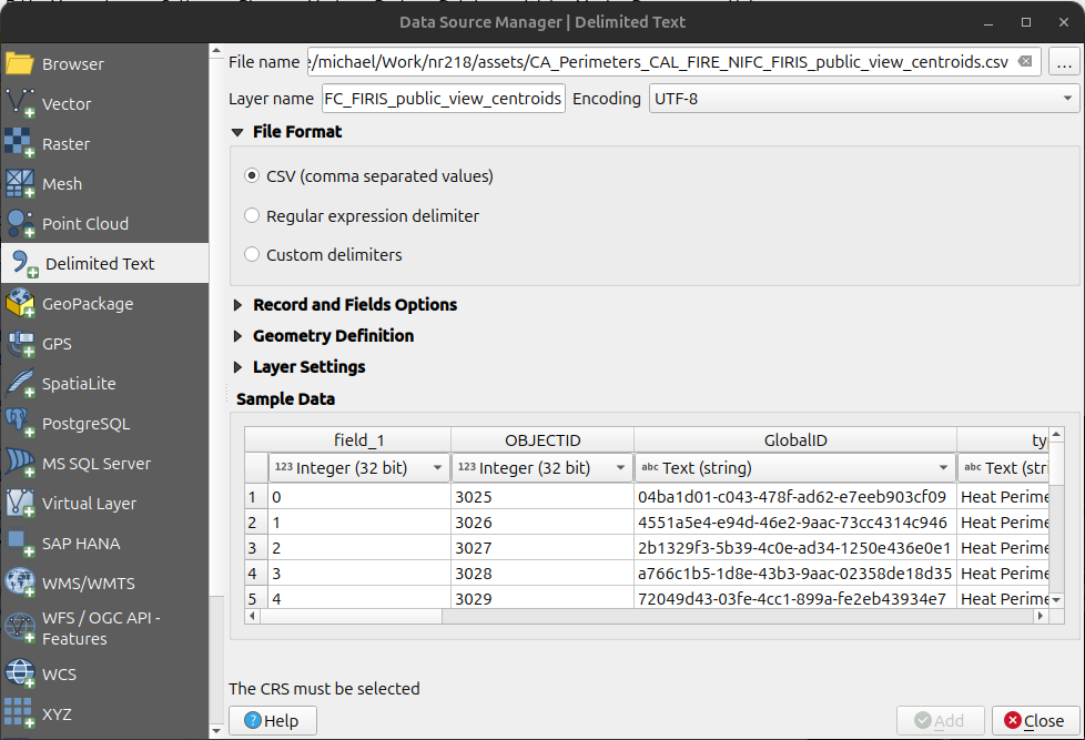
Delimited text dialogue box
Browse for csv
Notice that it says CRS must be selected.
What is a CRS?
- We will discuss what a CRS is in great detail later.
- For now just know it provides a reference frame for placing the coordinates on the map.
- Coordinate Reference System (CRS) is synonymous with Spatial Reference System (SRS)
- SRS = CRS
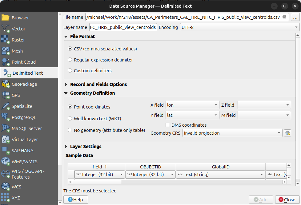
Click the Geometry Definition dropdown to assign an SRS.
Use EPSG:4326 - WGS 84
Click Add
Levels of Measurement
- Nominal - Names or identifiers of objects
- Ordinal - Ranked categories based on a measure
- Ratio - have a 0 value that indicates absence of the quantity of interest
- Interval - have a regular scale, but not a meaningful 0 value
Nominal - Names or identifiers of objects
e.g. Land Cover: “Oak Woodland”, “Grassland”, “Forest”, etc…
Ordinal - Ranked categories based on a measure
e.g. Fire Hazard: “Low”, “Medium”, “High”
Ratio - Multiplication makes sense, e.g. 200 K is twice as hot as 100 K \[ 2 \times 100 \mathrm{K} = 200 \mathrm{K} \]
Interval - Multiplication does not make sense, e.g. 200°C is not twice as hot as 100°C \[ 2 \times 100°\mathrm{C} \neq 200°\mathrm{C} \]
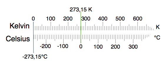
Image Source: wikimedia
Geospatial Data Types: Vector vs. Raster
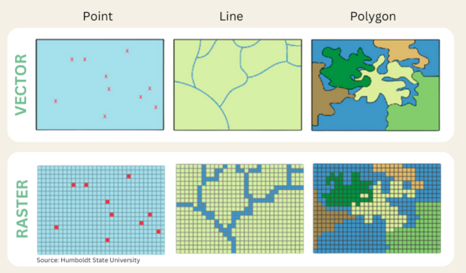
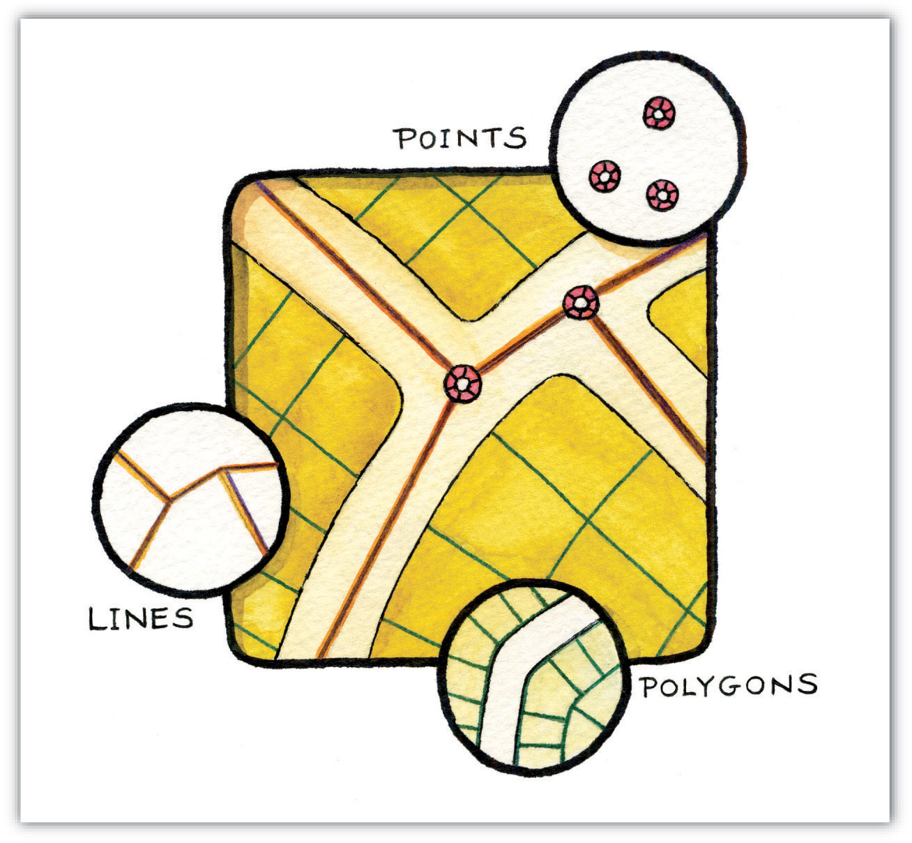
Vector Data
- Can be described by points, lines, polygons
- Ex: roads, rivers, train tracks, hiking trails, sidewalks, building footprints, county boundaries
- NOT images, do NOT contain any pixels
- The kind of data we’ve been working with so far
- Often stored as tabular data files with geographic metadata
- Points, lines, and polygons represent the spatial features
- Topology describes the connectivity, area definition, and contiguity of interrelated points, lines, and polygon
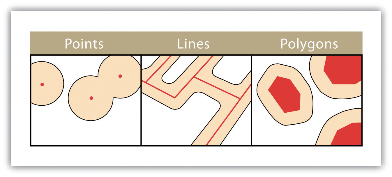
Points
- Zero-dimensional objects containing a single coordinate pair.
- Ex: Lat, Lon (sometimes elevation) coordinates denoting a city, building, address, etc
- X,Y (,Z) coordinates on a Cartesian plane (or Euclidean space)
Lines
- One-dimensional objects composed of multiple, explicitly connected points.
- Lines have the property of length.
- Also called an “arc.”
Polygons
- Two-dimensional features created by multiple lines to create a “closed” feature.
- First point on the first line segment is the same as the last point on the last line.
- Can represent city boundaries, buildings, lakes, soils, etc.
- Have the properties of area and perimeter.
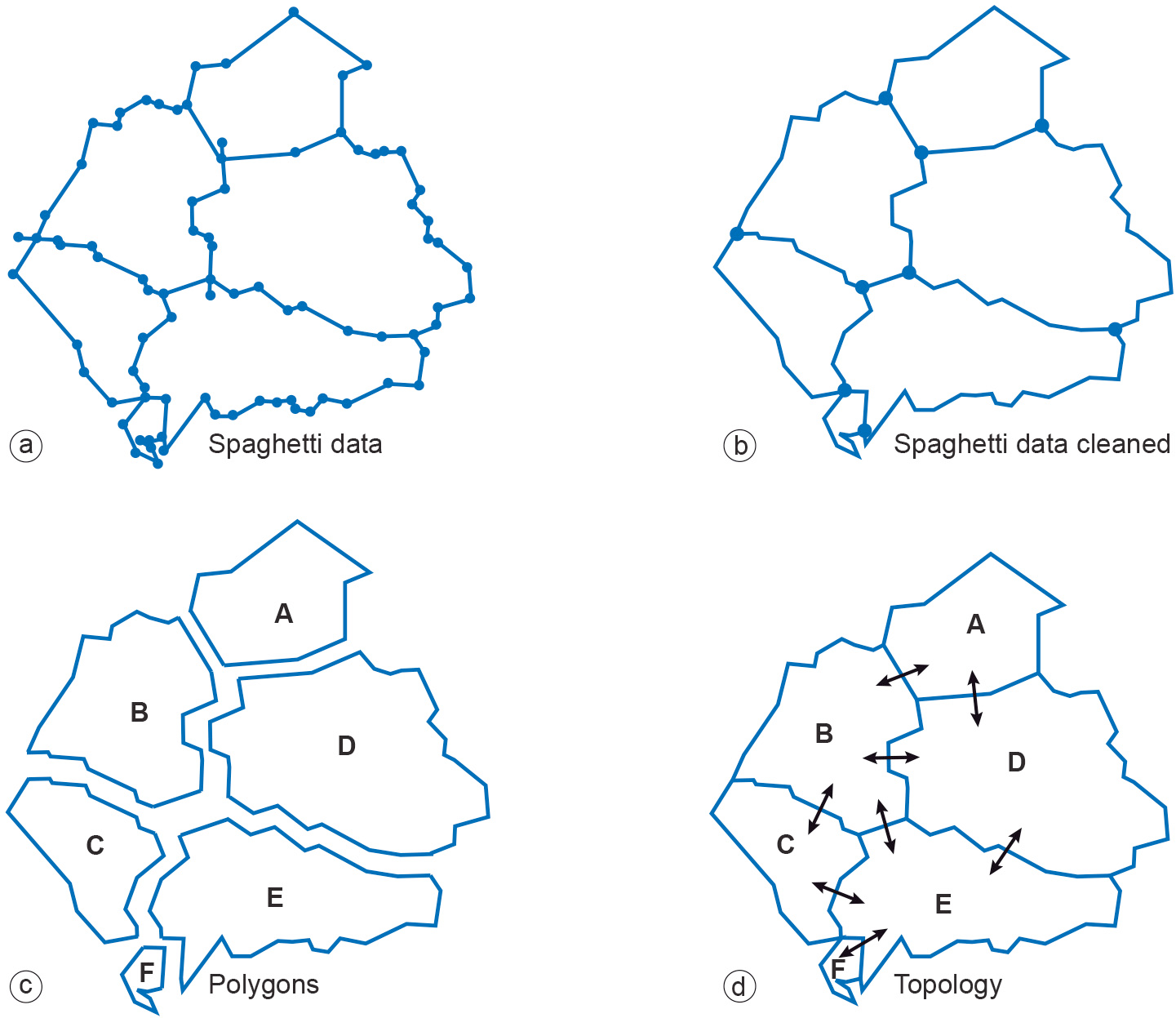
Structuring Vector Data
- There are several ways to define relationships between vector data:
Feature based: The “Spaghetti Model”
- Each feature is a long string of coordinates
- No relationships between features
Structured: The “Topological Model”
- Enforced relationships between features
Raster Data
Raster Data
- Derived from a grid-based system of contiguous cells containing specific attribute information.
- The spatial resolution of a raster dataset represents a measure of the precision or detail of the displayed information.
- Widely used by technologies such as digital images and LCD monitors.
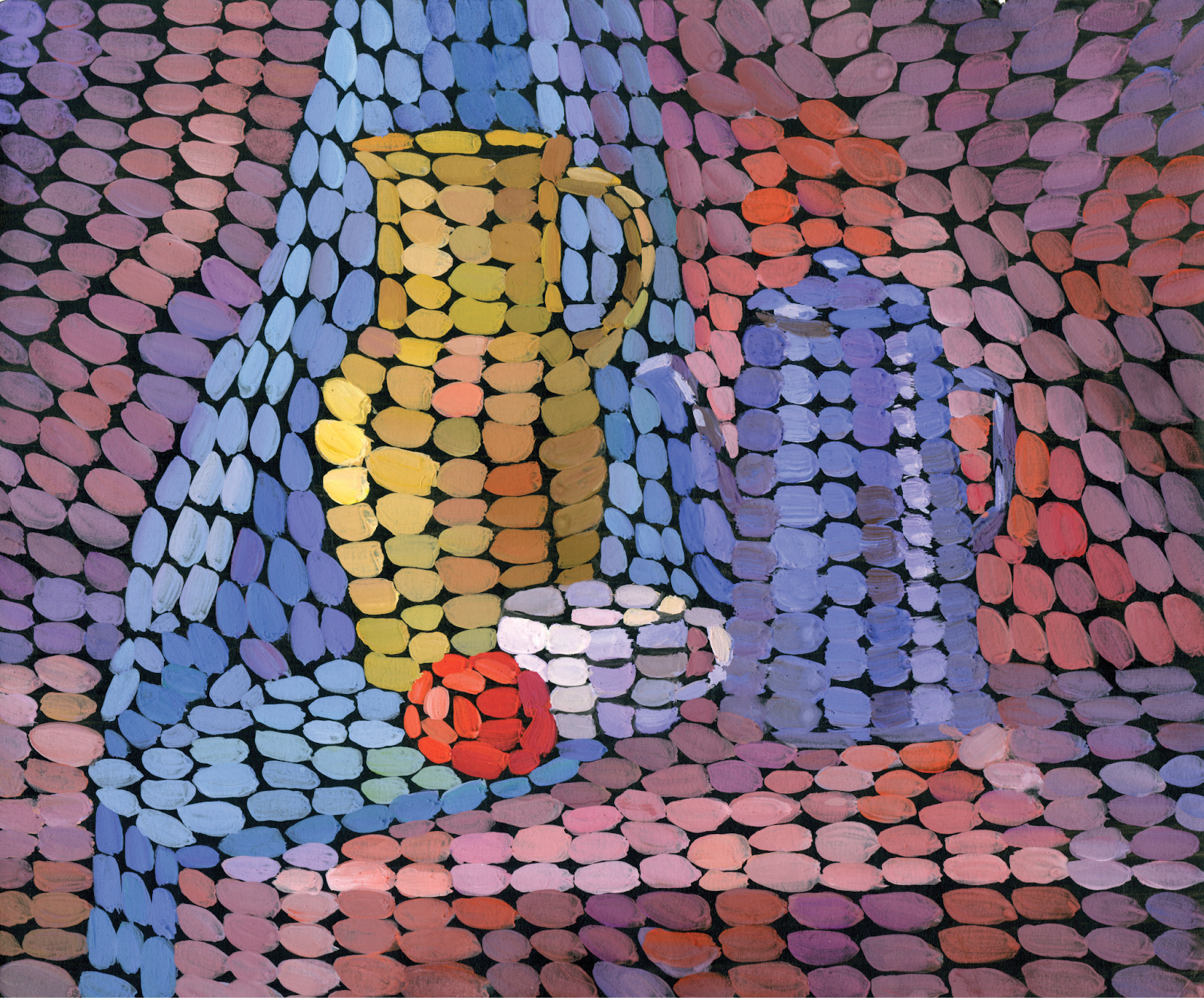
- Images, stacks of images (satellite / drone image)
- Rastrum, Latin meaning “scraper” –> Raster, German meaning “screen”
- Grids of numbers
- Things with pixels!
- If it’s pixelated:
- It’s a raster
- If it’s a photo:
- It’s a raster
- If it’s a digital image
- It’s a raster!
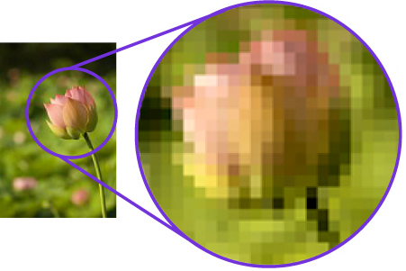
- The spatial resolution of a raster dataset represents a measure of the precision or detail of the displayed information.
- a.k.a. pixel size
- Ex: 1mm, 1cm, or 1m
- So when you hear that a camera has N megapixels - this just means it has many millions of pixels
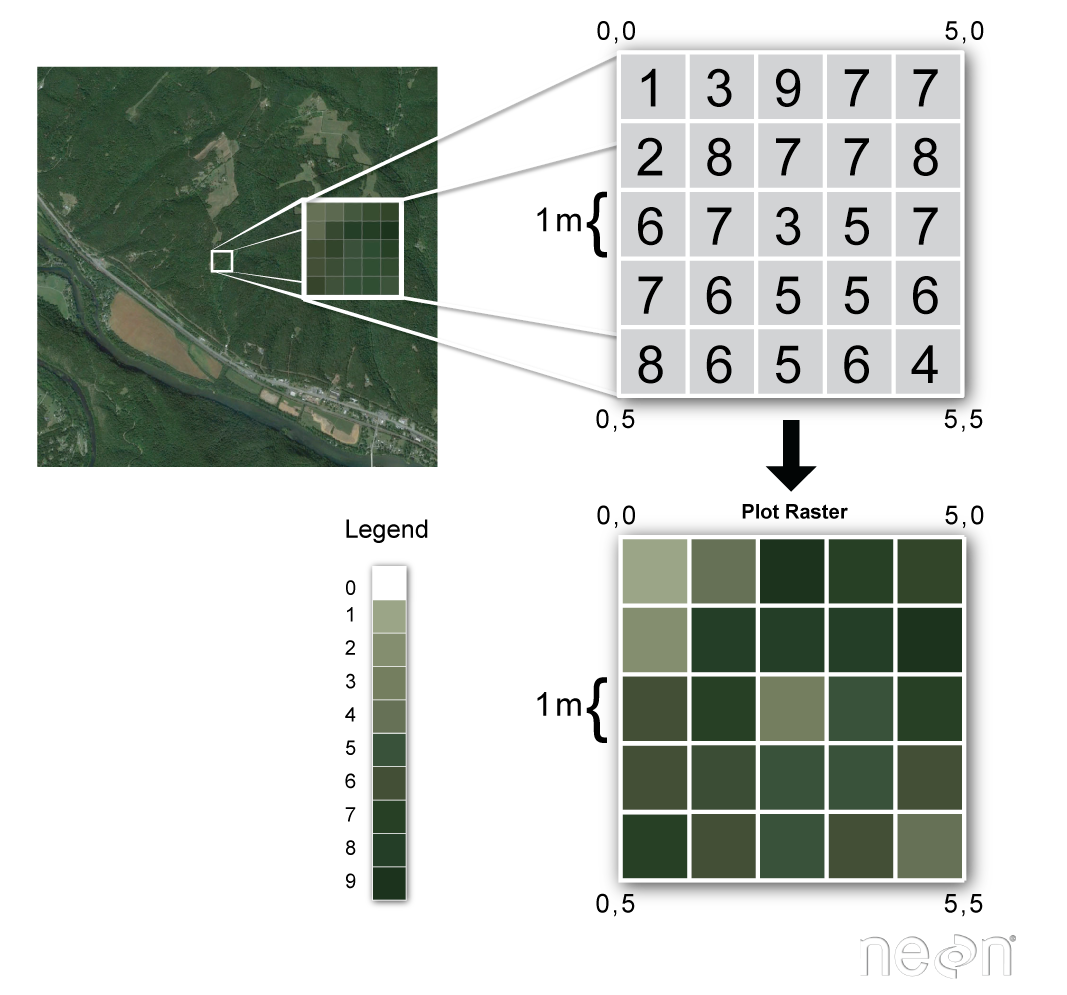
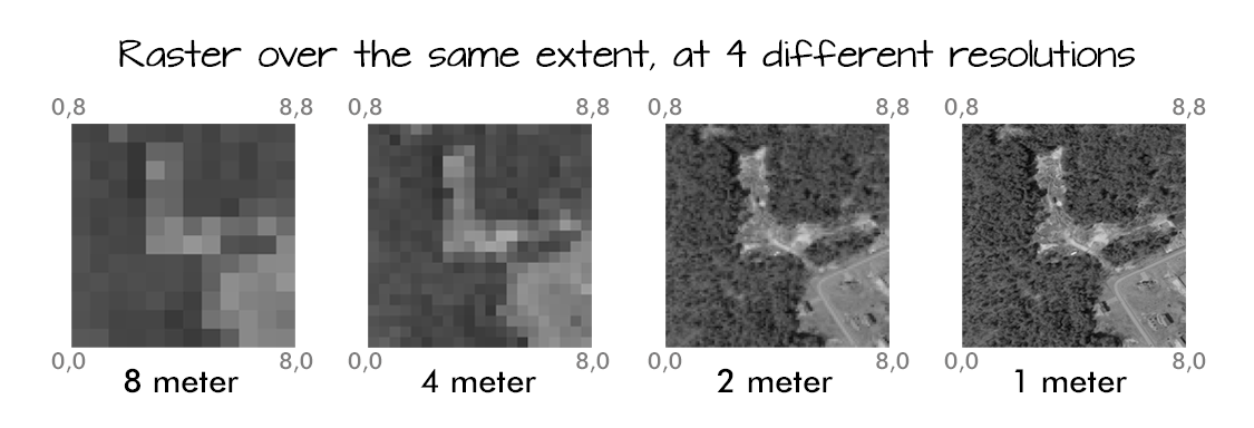
Spatial Resolution
The spatial resolution of a raster dataset represents a measure of the precision or detail of the displayed information.
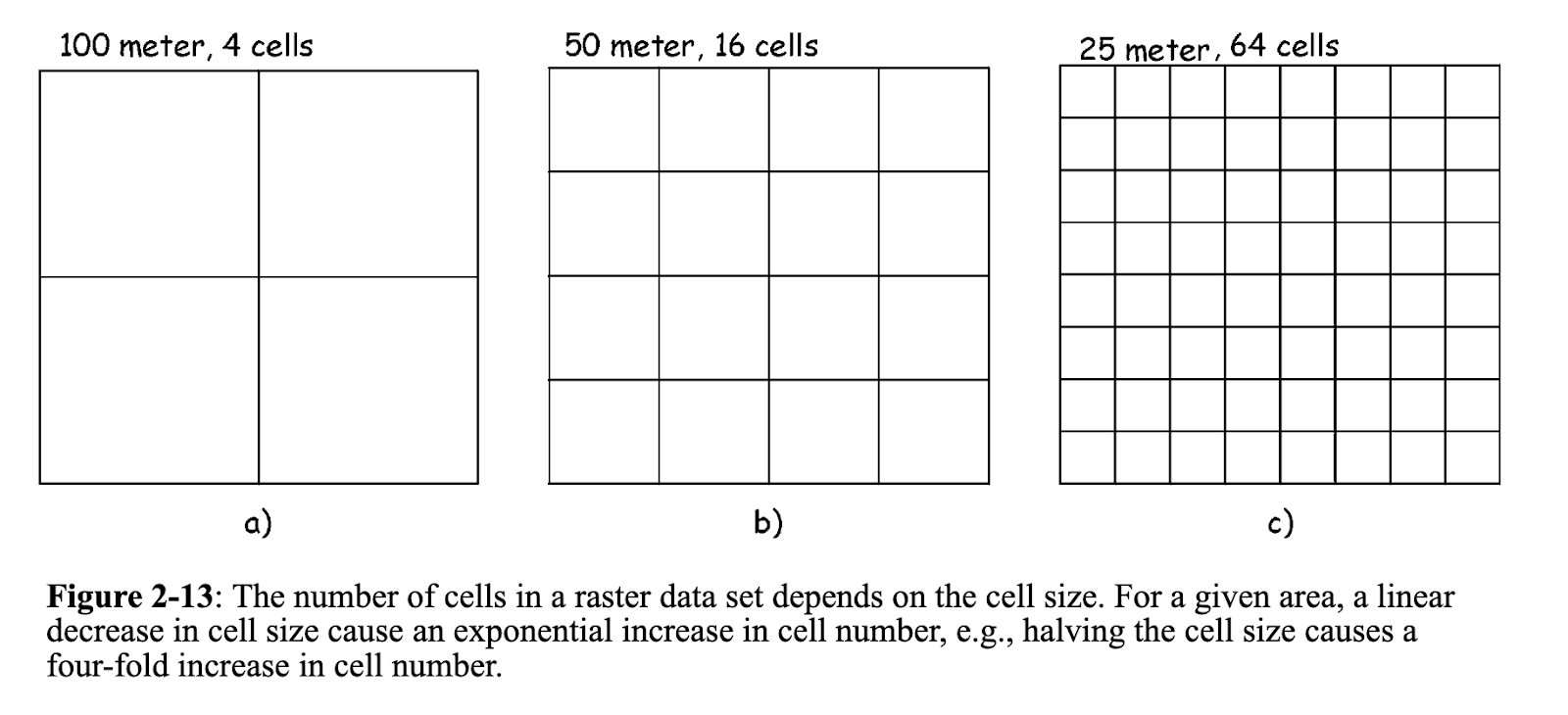
The spatial resolution of a raster dataset represents a measure of the precision or detail of the displayed information.
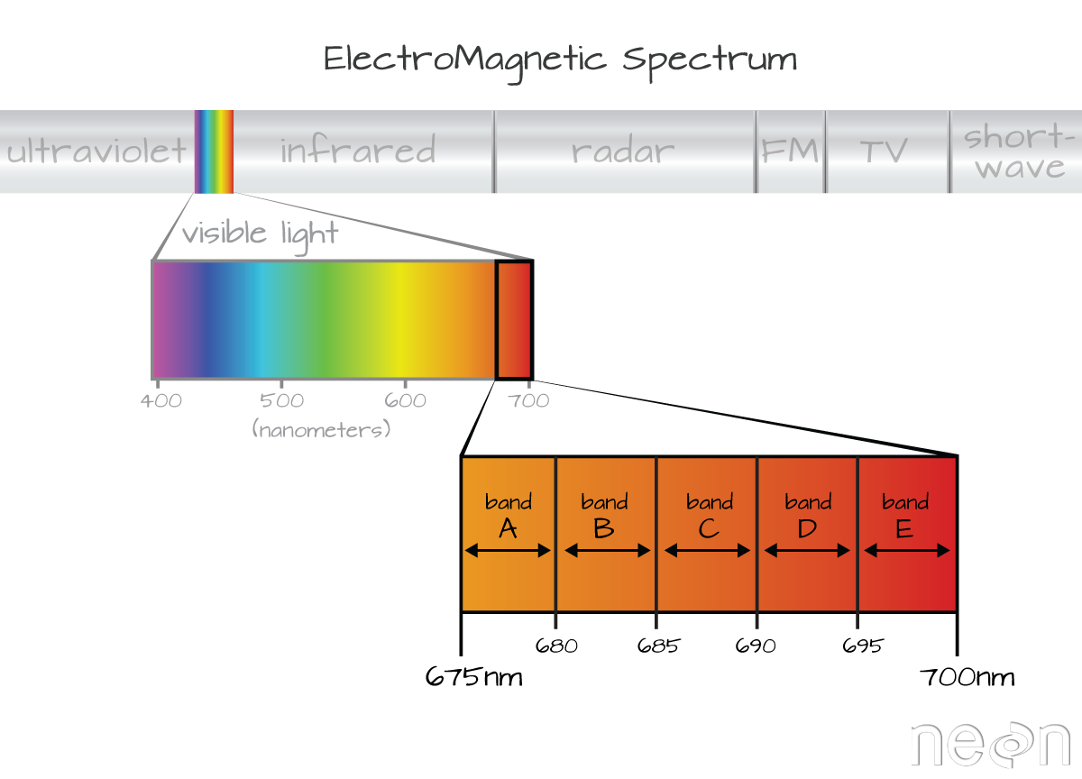
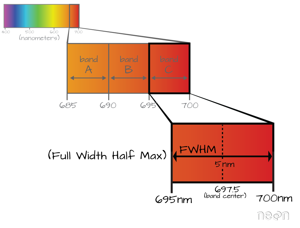
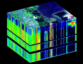
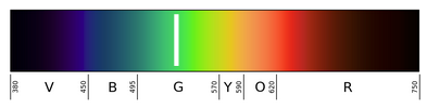
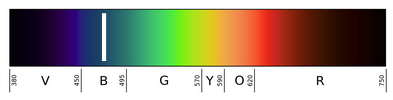
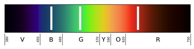
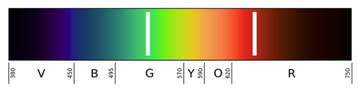
Spectral Resolution
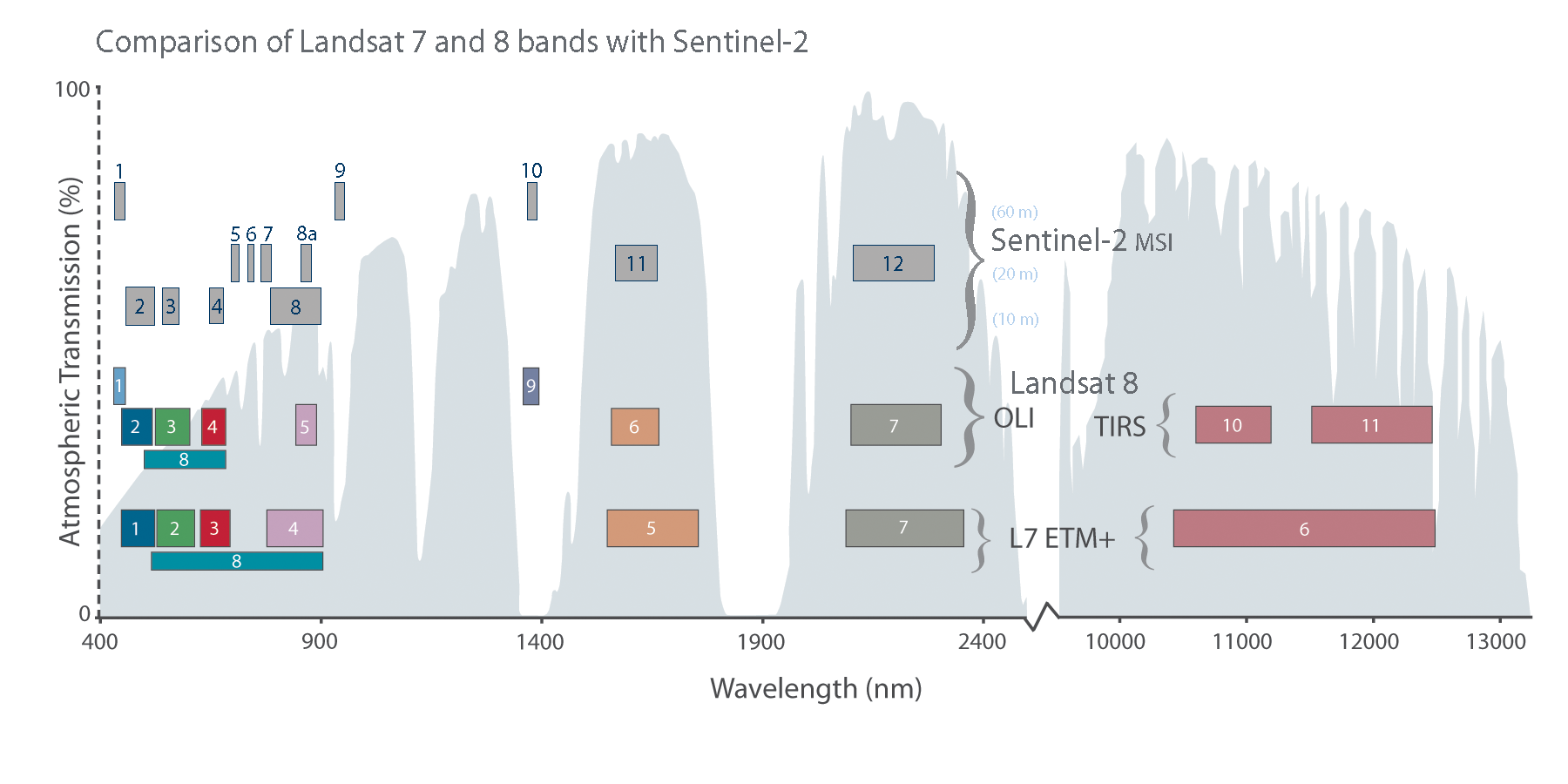
What is Sentinel 2
Sentinel 2 is a mission run by the Copernicus Programme (the EU Space Program’s Earth observation component)
- Multispectral imagery
- Multiple Satellites 180 \(\deg\) out of phase with one another
- 5 day revisit (at equator)
- Wide swath width (290 km)
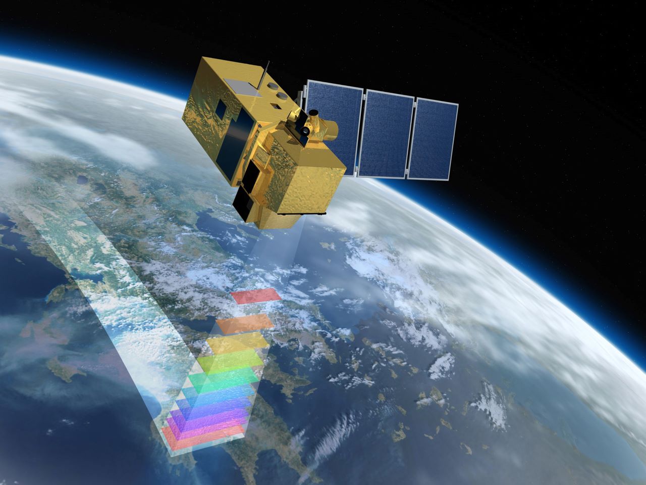
Image Source: Copernicus
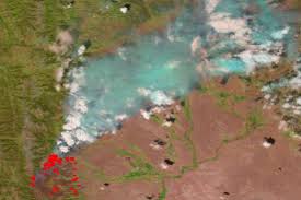
Oil Spill detection
\(OSI = \frac{1}{3} \times \frac{Green + Red}{Blue}\)
Another common combination
\(B3 + B8 + B11\) or \(Green + NIR + SWIR1\)
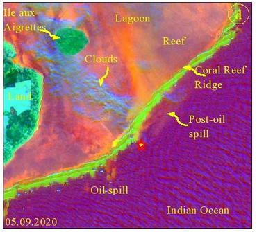
Image Source: Sentinel Hub
Similarity to Landsat
| Satellite | Spatial resolution | Number of bands | Revisit time |
|---|---|---|---|
| Sentinel-2 (A/B) | 10 m, 20 m, 60 m (band-dependent) | 13 | 5 days (with both satellites) |
| Landsat (8/9 OLI/TIRS) | 30 m multispectral, 15 m panchromatic, 100 m thermal (resampled to 30 m) | 11 | 8 days (with Landsat 8 + 9; 16 days each alone) |
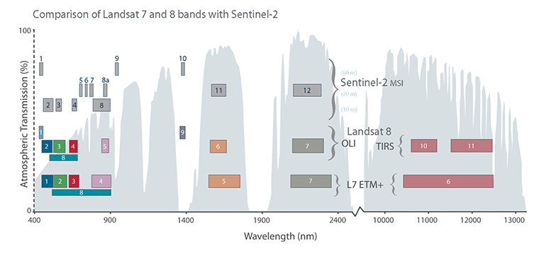
Image Source: Copernicus
You should see something like this when it first opens:
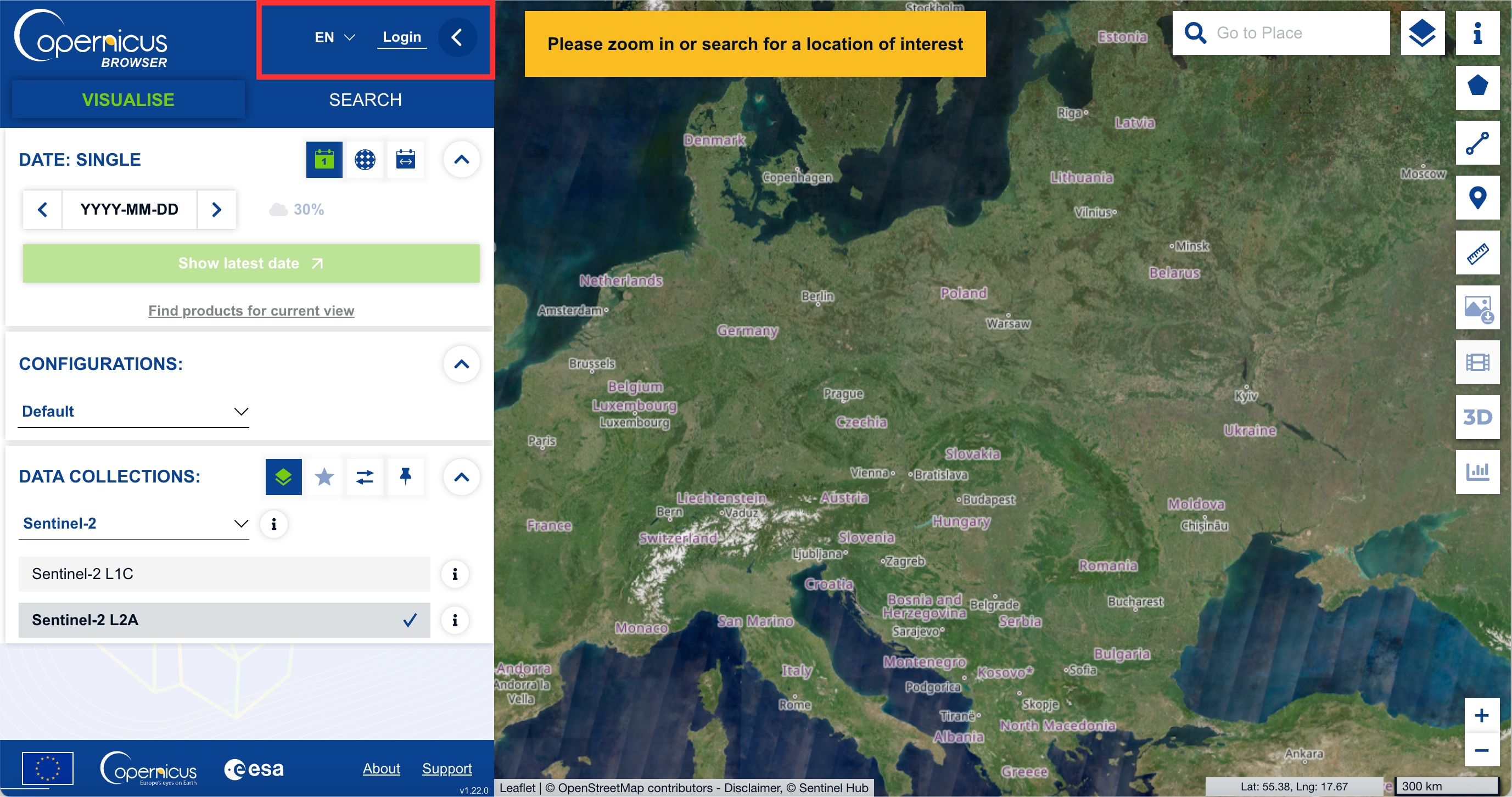
To register, click the “Login” button at the top of the left panel
Follow the steps to register, confirm your email, and then go back to the main page.
Look at the Garnet Fire on CalFire inciweb.
- In Copernicus Browser (in visualize mode), paste the lat, lon into the search, hit enter
- Change the date to 2025-09-07
- Adjust image so the fire is in view
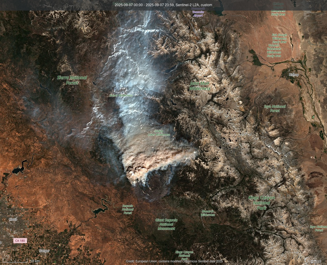
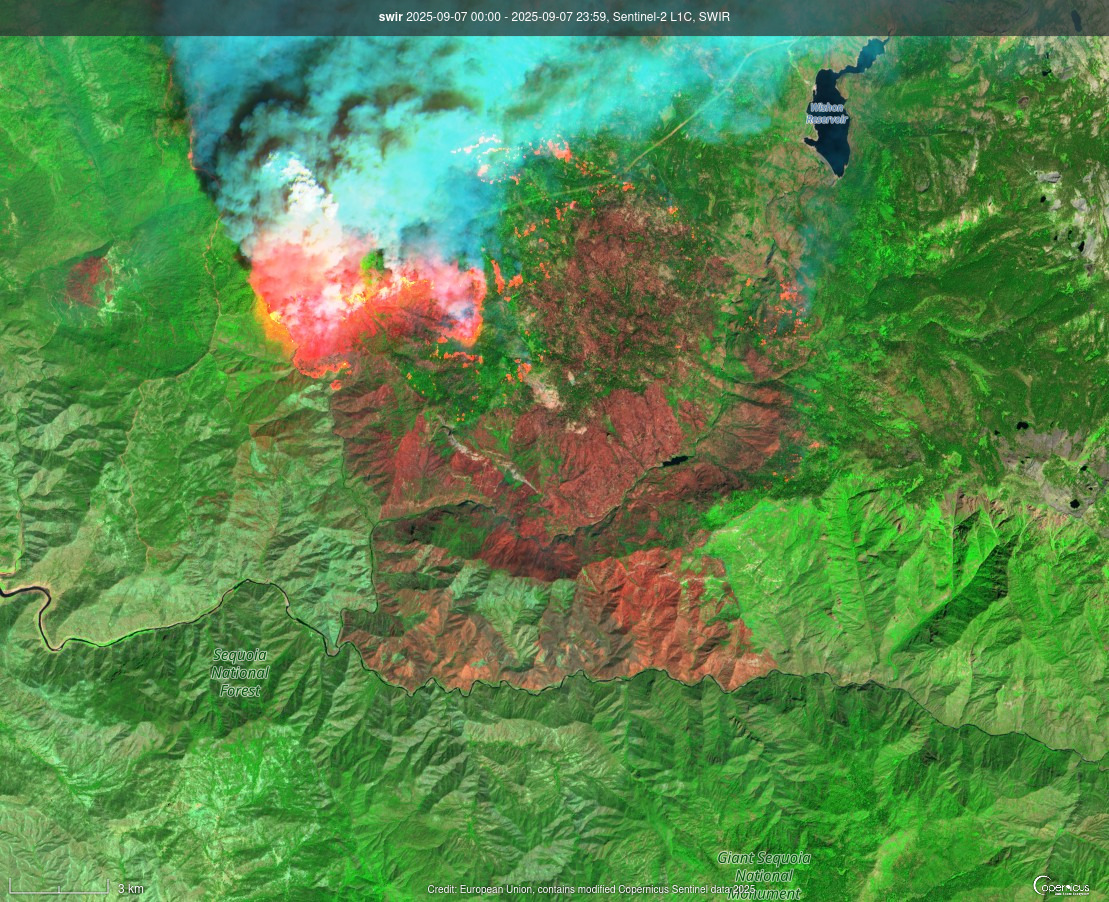
- Lets try a different visualization
- Copernicus offers a SWIR based composite visualization that is quite good for burn detection.
Step One - Registering for GEE
- To connect your Google account, go to https://code.earthengine.google.com/
- Once you’ve logged in, you should see something like this:
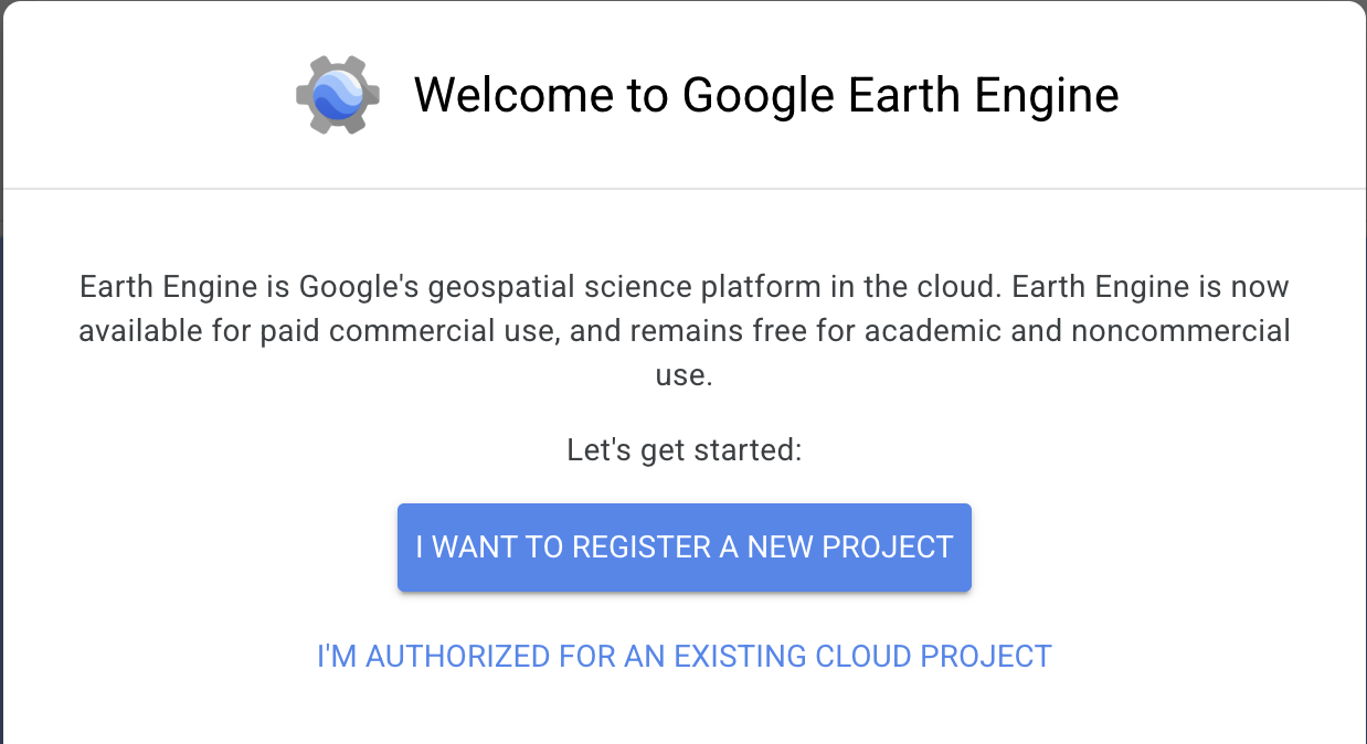
- We want to register a new project
- Name your project something useful, then hit create
- Next, we want to register the project for non-commercial use
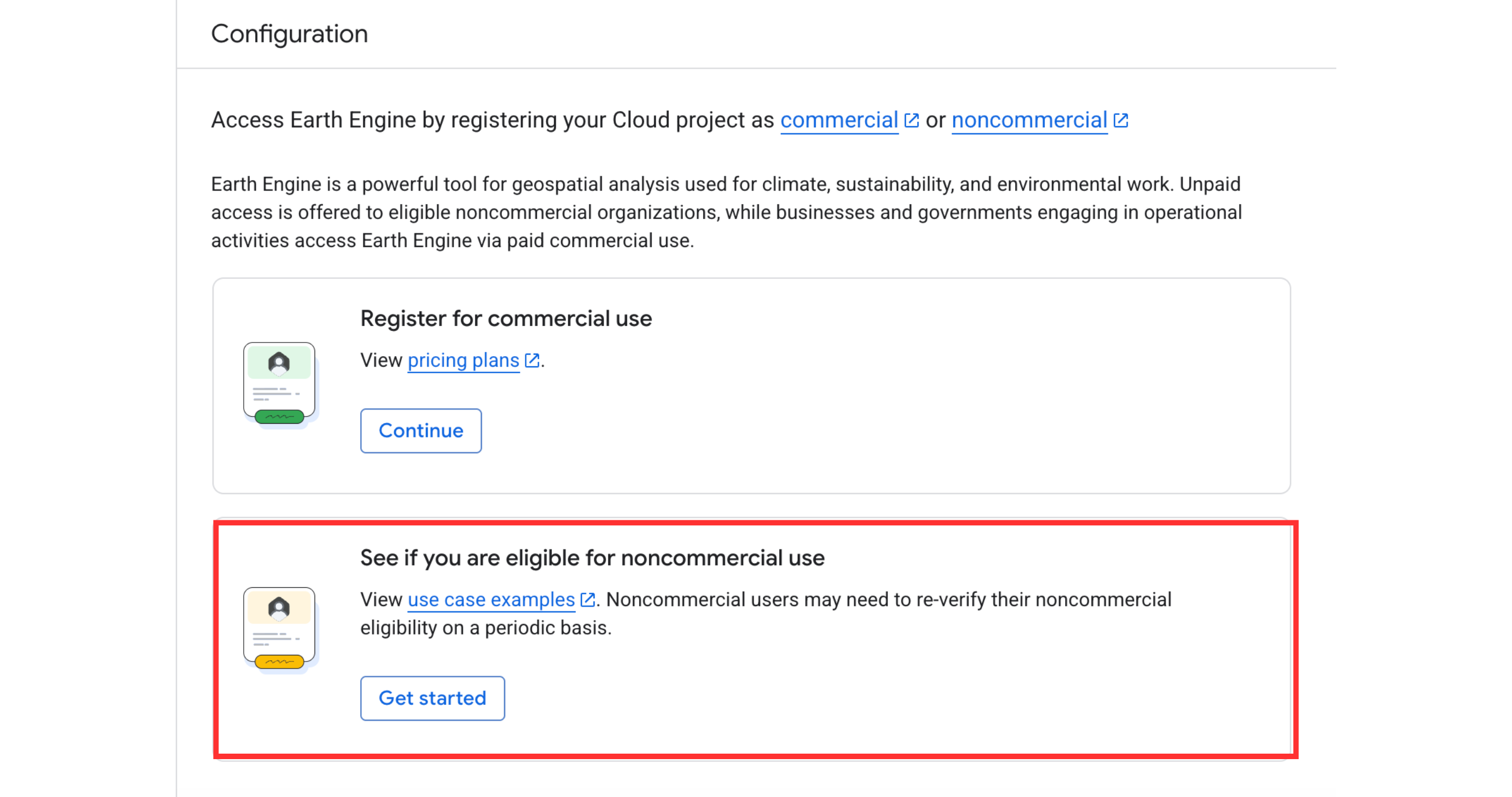
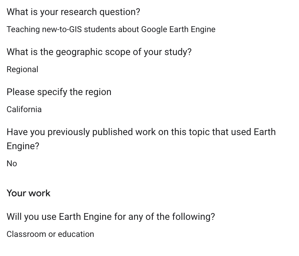
This will take you to a form where you can confirm your eligibility. Here’s an example of how to fill it out:

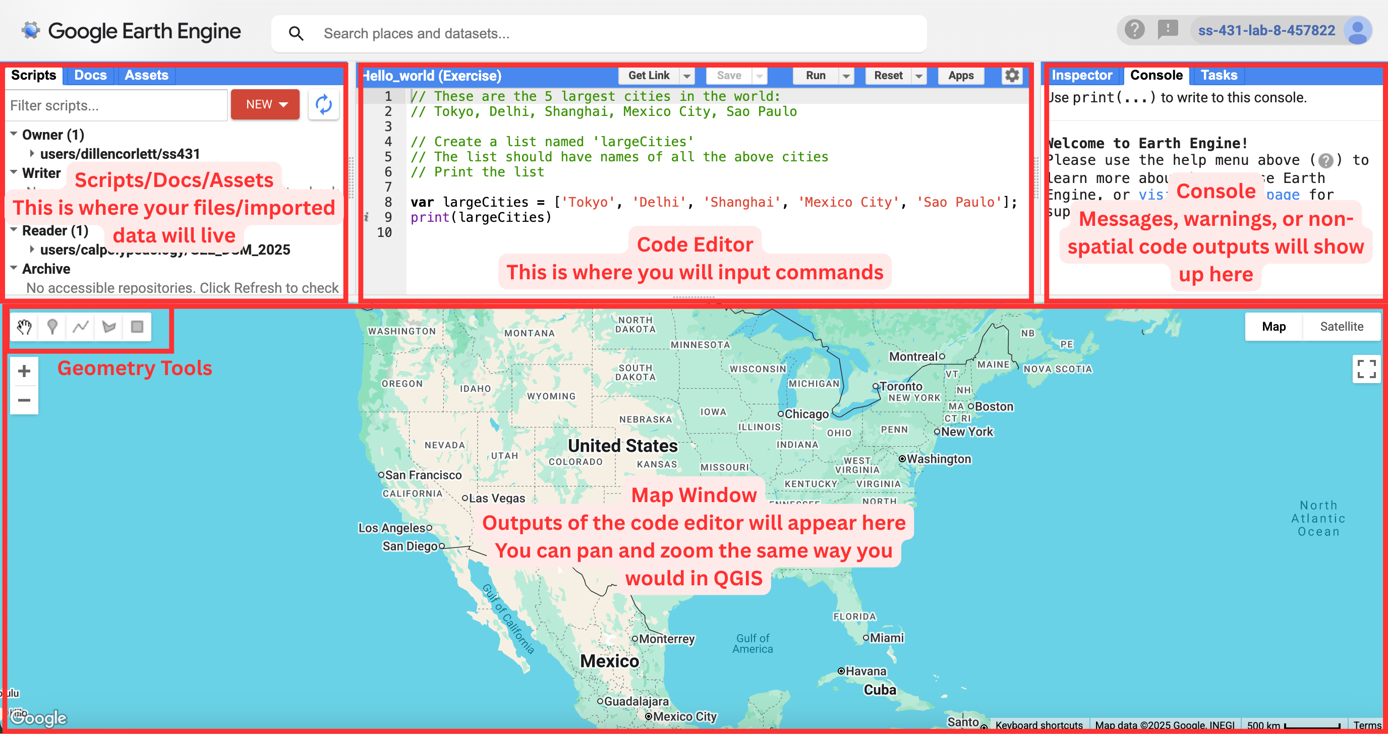
These are the main panels to be aware of:
Step Two - Editing and Running a Script
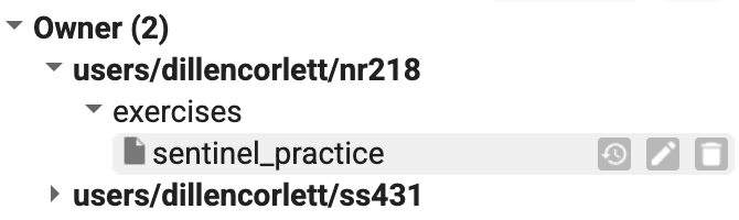
- In the scripts panel, select New > File and name it something useful
- You should see it show up under the Owner dropdown:
- Click on the file to open it, and then move to the Code Editor. It should be blank to start.
- Let’s try running some code! In the editor window, type the following command:
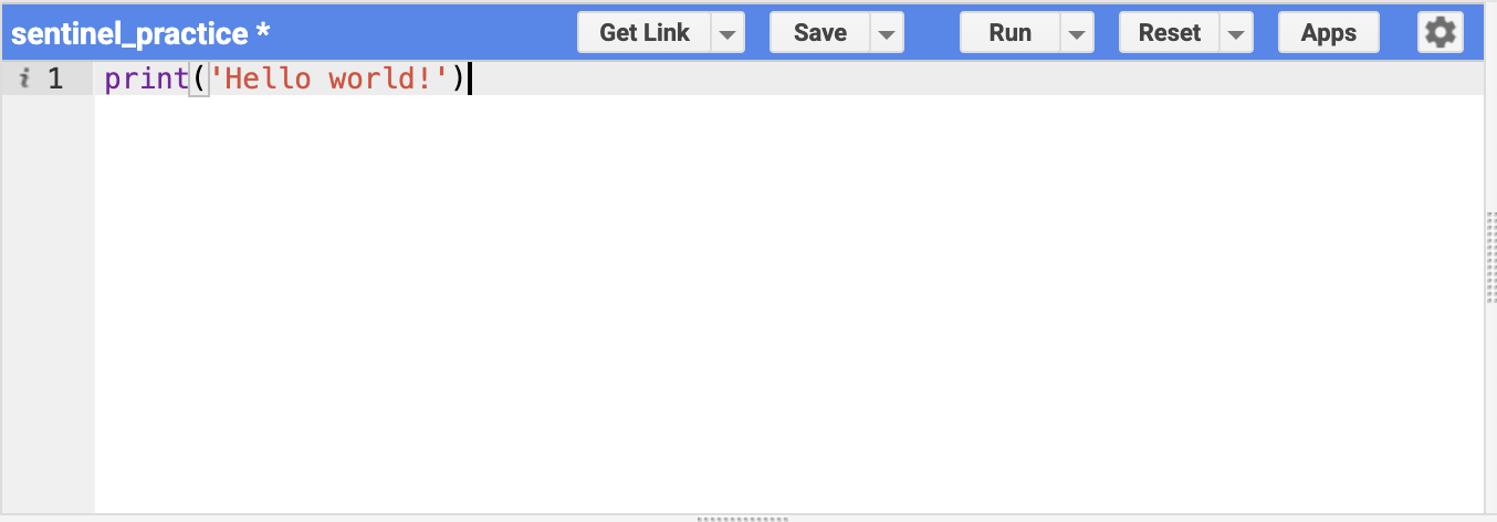
- Then hit run. Look at the console - what do you see?
Next, we’re going to explore some spatial data.
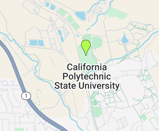
- In the search bar at the top of page, type in “California Polytechnic State University”
- Click on the search result, and the map view should update accordingly
Add a marker to the map by clicking this icon:
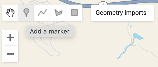
Place the point somewhere in the middle of campus:
- At the top of the code editor, you should now see a new var called “geometry”, which gives us the coordinates of our point
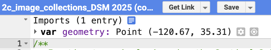
- We can now reference the point in new lines of code, like we did with “largeCities”
- To add in other data layers, let’s look in the Earth Engine Data Catalog
- Using the search bar, find the Sentinel-2 Dataset and click on the Level-1C option
- Scroll down to the “Explore with Earth Engine” section, and copy the JavaScript code
- Go back to the code editor, and paste the code onto a new line
Before we run it, let’s make a few changes to the code.
- First, let’s change these dates to be more recent:
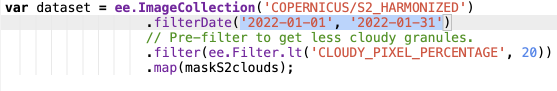
- Pick a month in 2025, and set the dates to be the first and end of the month
- Next, let’s change the center point of the map to the point we dropped earlier:
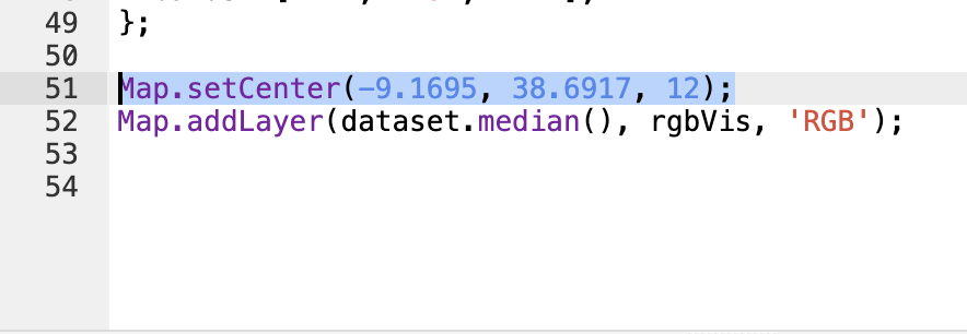
- Replace the entire line with the following code:
- Alternatively, you can just replace the first two numbers with the coordinate values saved to “geometry”
Hit run, and watch what happens in the map viewer! It may take a second for the layer to load.
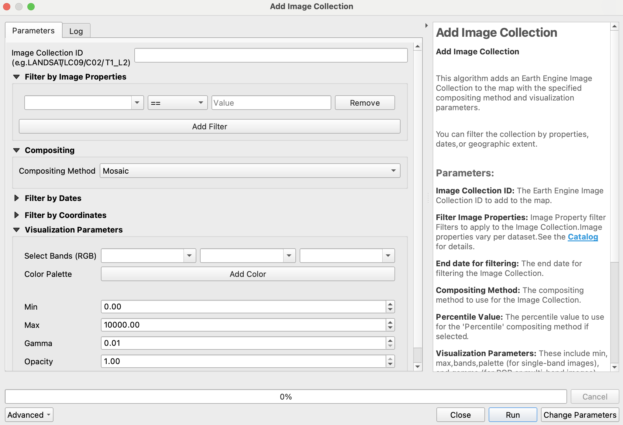
We can do the same operation we just did through the plugin:
Vector Data (Review)
- Can be described by points, lines, polygons
- Ex: roads, rivers, train tracks, hiking trails, sidewalks, building footprints, county boundaries
- NOT images, do NOT contain any pixels
- Often stored as tabular data files with geographic metadata
- Points, lines, and polygons represent the spatial features
- Topology describes the connectivity, area definition, and contiguity of interrelated points, lines, and polygon
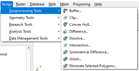
Buffer
- Open QGIS and open the ‘sprStreams.geojson’ from the SPR data we used the other day. (If you do not have it any longer it can be downloaded here)
- In the drop down menu go to, Vector –> Geoprocessing tools –> Buffer
Notice the Units! Buffering in degrees makes no sense. Reproject it first! What is a good projection to use?
 {fig-alt=“QGIS warning about buffering in degrees”, width=“30vw;”}
Dissolve
- In QGIS open
sprSoil.geojson - Change symbology to categorical by “SOILNAME”
- Vector –> Geoprocessing tools –> Dissolve
- Use “HYDROGRPOUP” as dissolve field
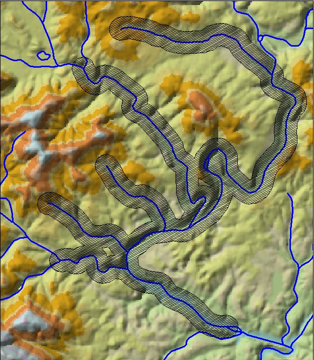
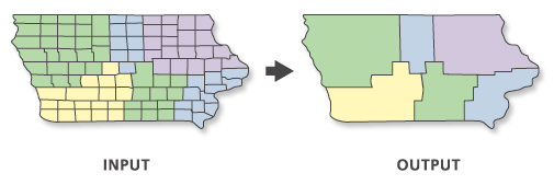
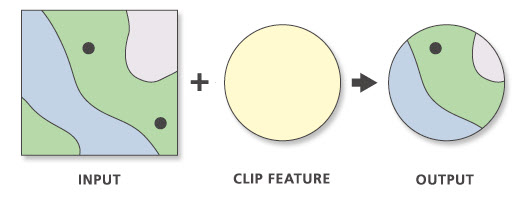
Clip
- Vector –> Geoprocessing tools –> Clip
- Clip the sprSoil by the streams buffer.
![]()
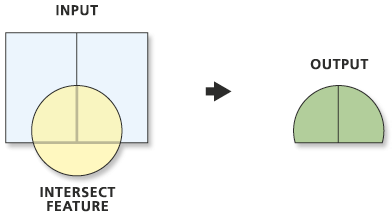
Spatial overlays
- Intersect soils with bufffer, look at attributes
- Intersect buffer with soils, look at attributes
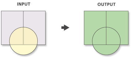
Union
Symmetric Difference
- Try it with buffer and soils
Joins
Tabular joins join layers by matching a common column name (e.g., parcel_id or GEOID)
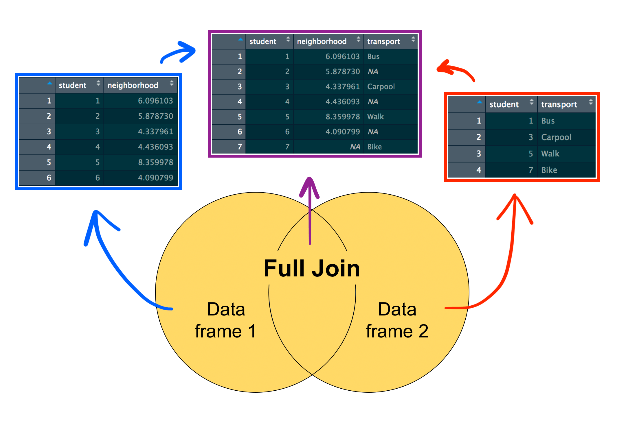
Spatial joins transfer attributes based on how features relate in space (intersects, within, nearest)
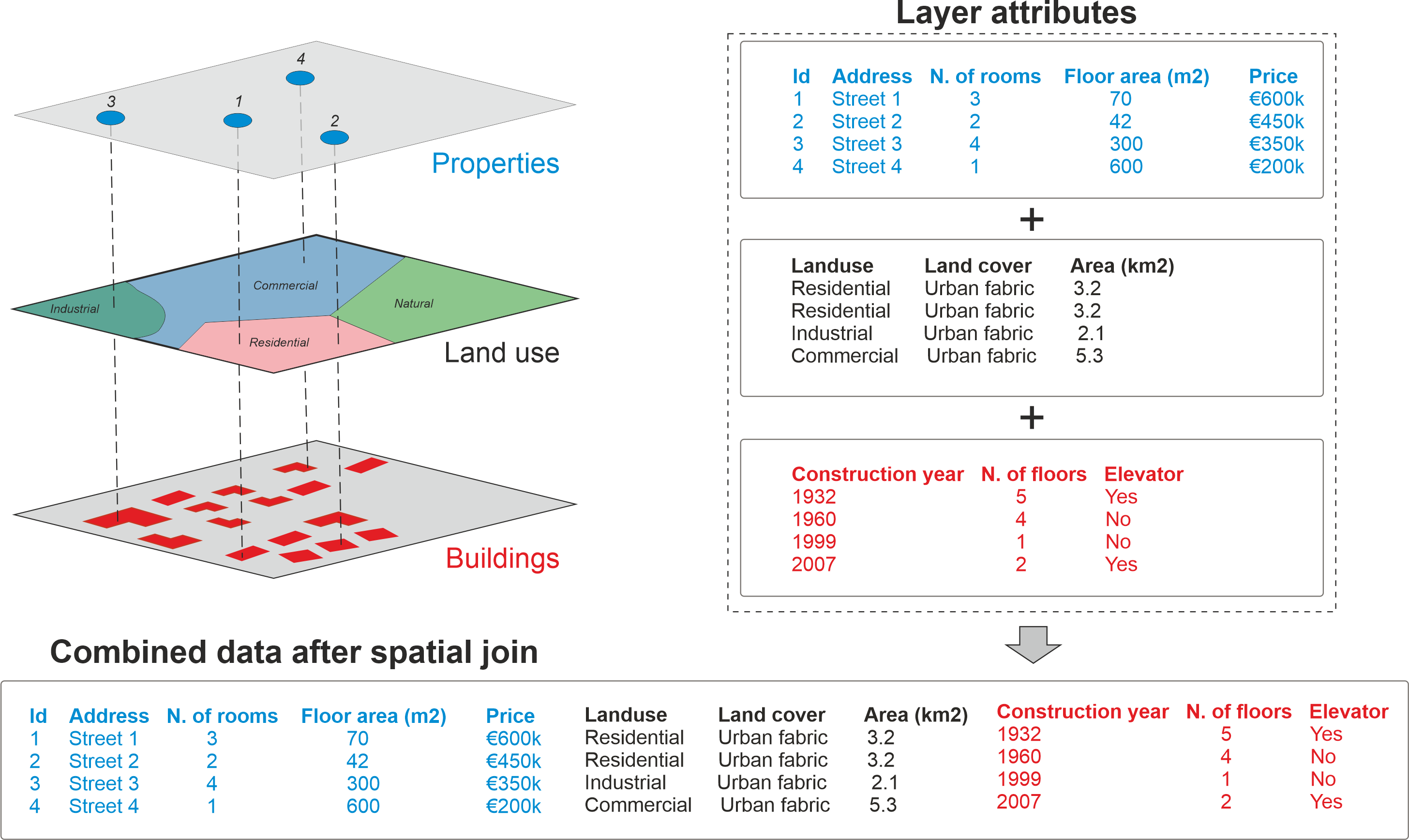
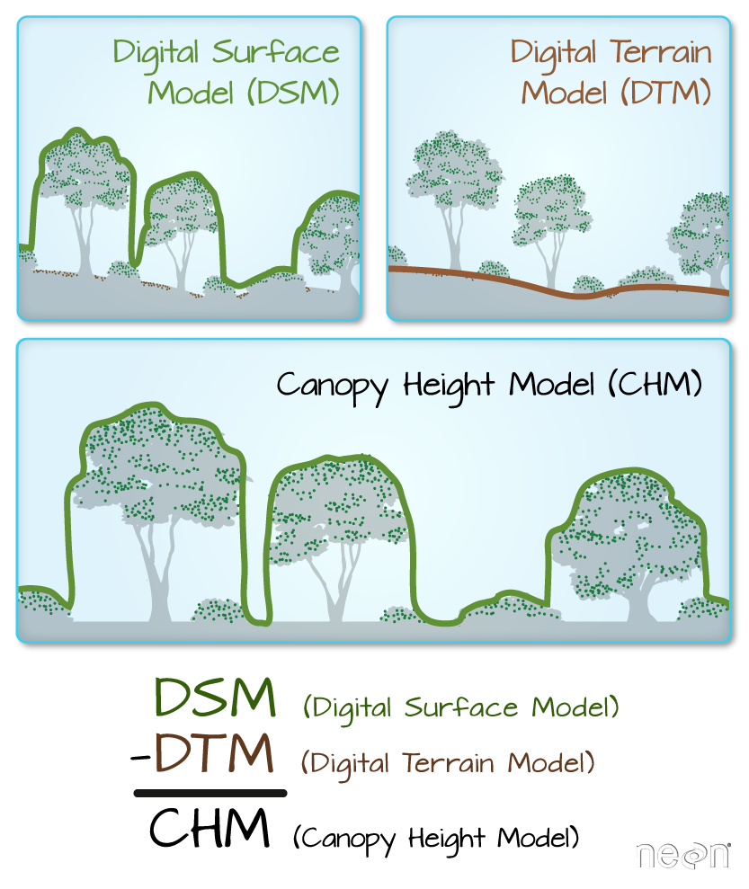
Image Source: NEON
How are DEMs made?
Satellite imagery
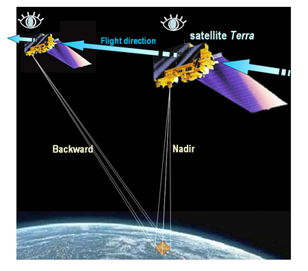
 Image Source:
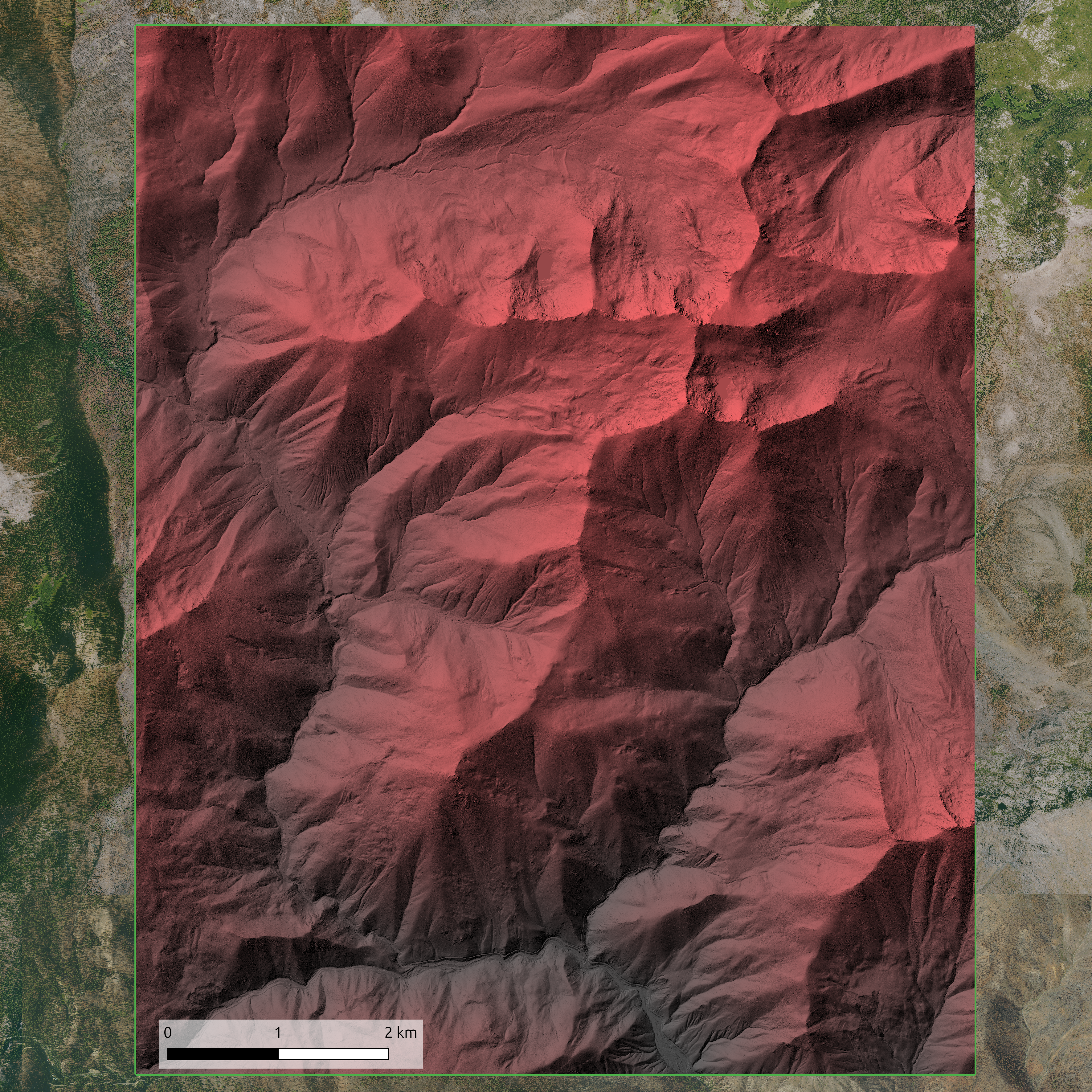
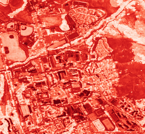
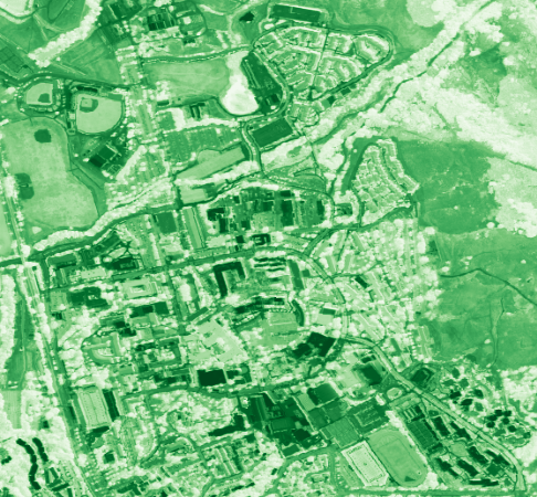
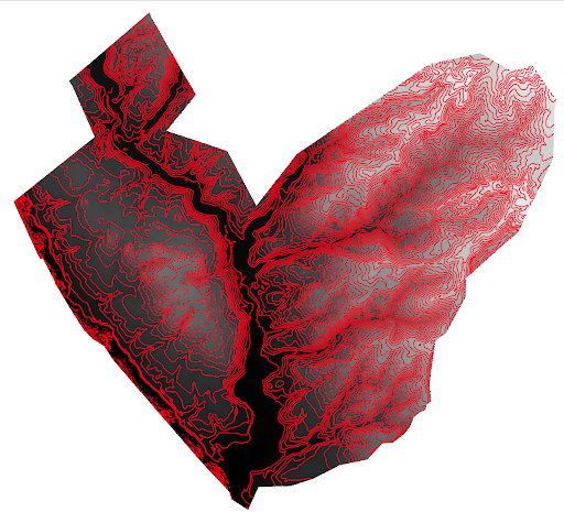
Visualizing Elevation
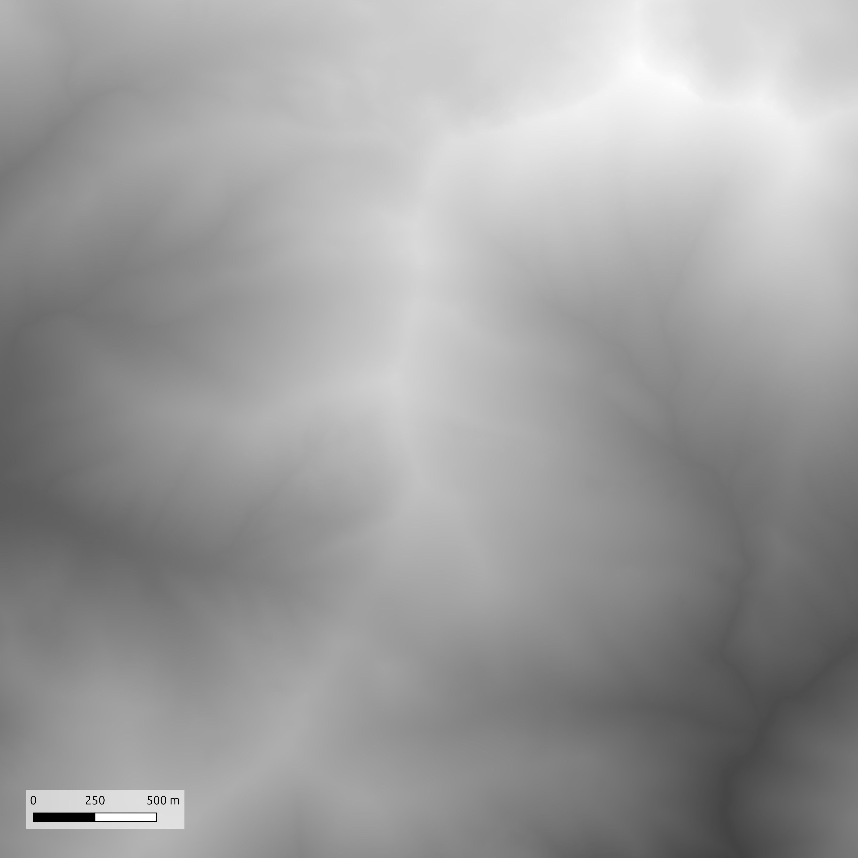
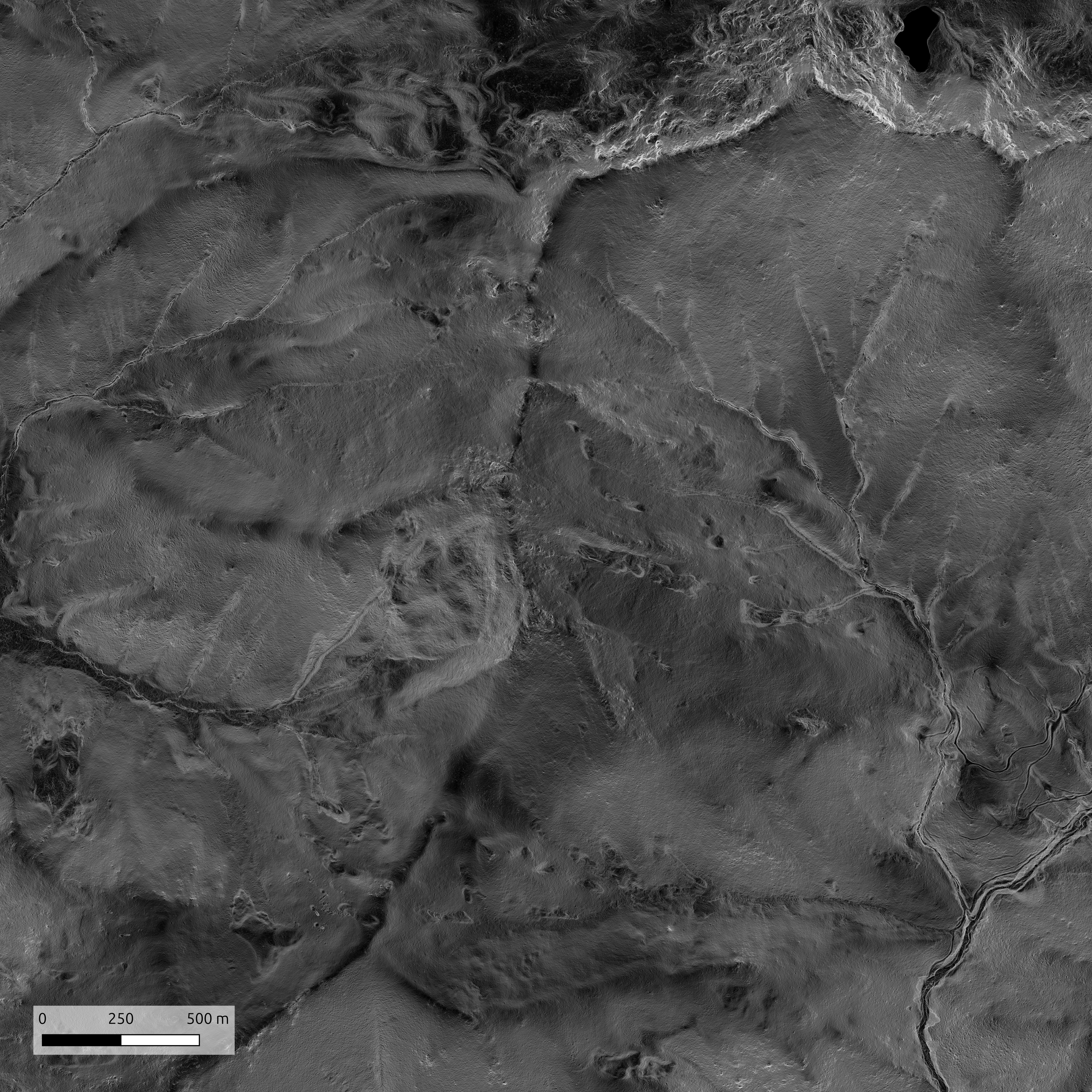
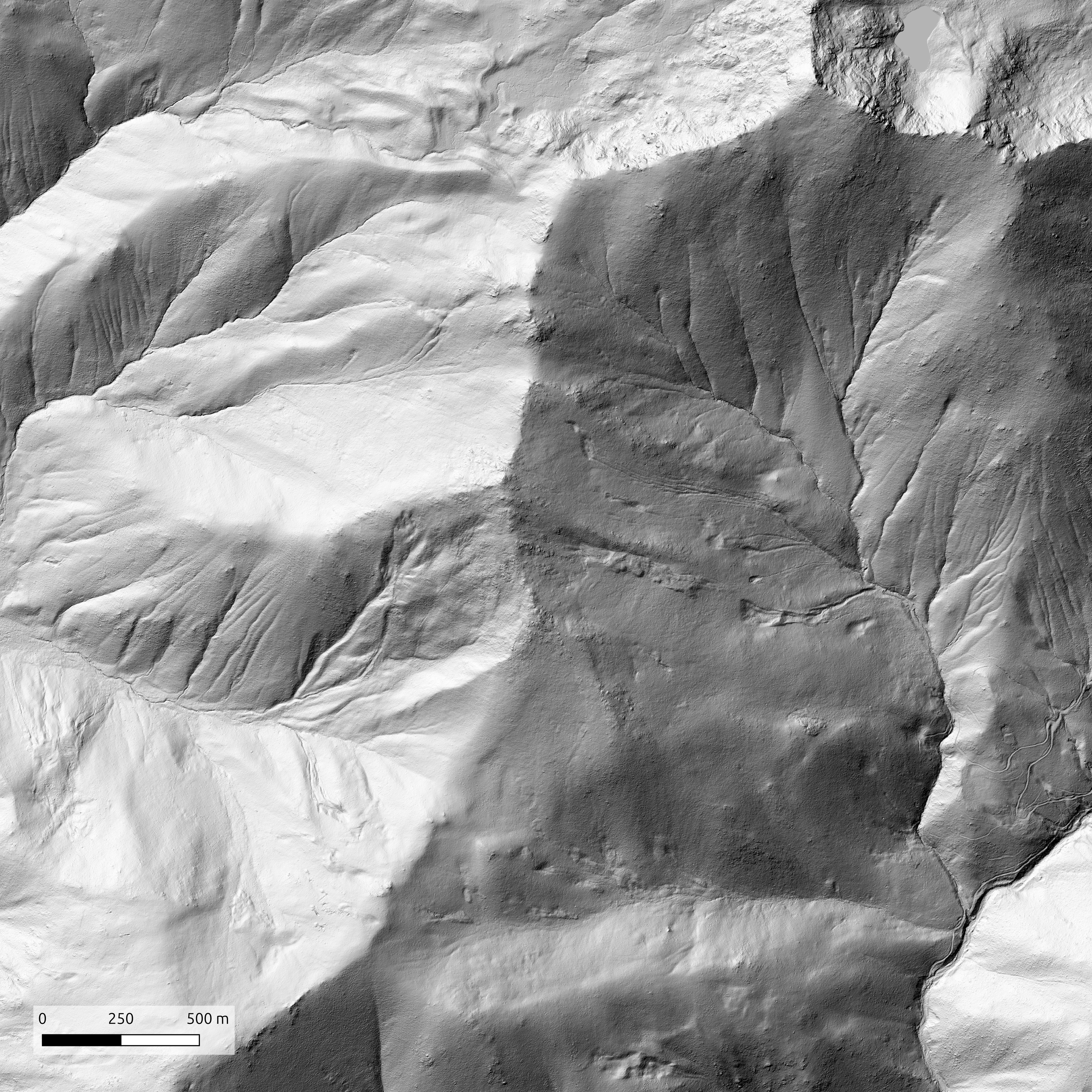
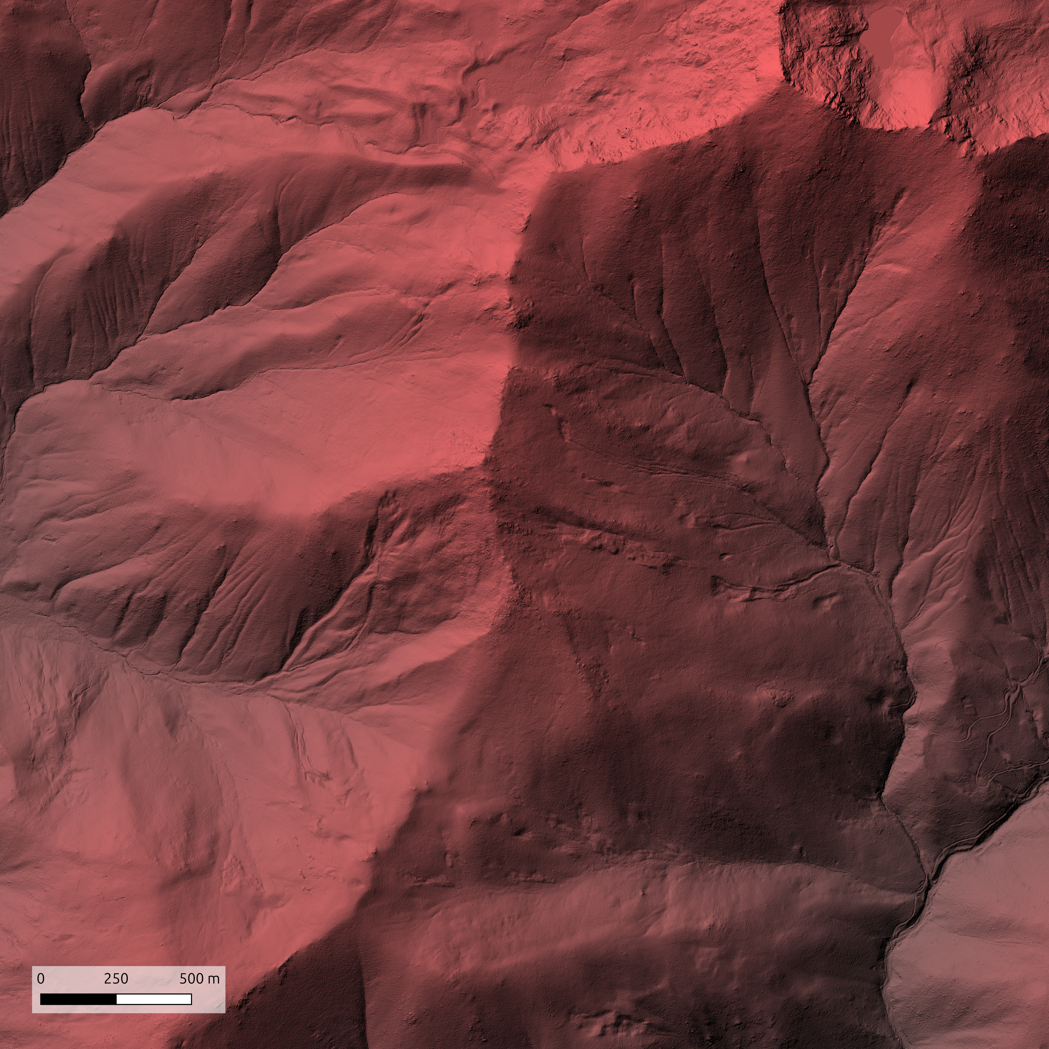
Red Relief
- Create Hillshade
- Raster → Analysis → Hillshade
- Azimuth: 315°, Altitude: 45°
- Apply Red Relief Style to DEM
- Right-click DEM → Properties → Symbology
- Render type: Singleband pseudocolor
- Color ramp: Create custom red gradient
- Min value: Black → Max value: Red
![]()
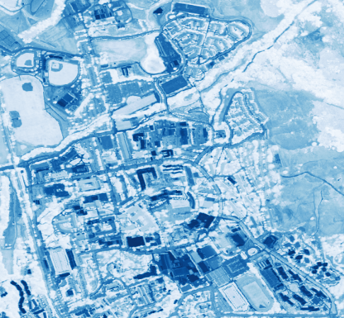
- Blend Layers
- Place hillshade above DEM
- Set hillshade Blending mode: Multiply
- Adjust hillshade opacity somewhere ~50-70%
- Opacity is found under the Transparency tab just below Symbology

Red Relief
Landforms
Raster Resampling
Resampling is adjusting the pixel size or resolution of raster data in order to:
- Match resolutions - So multiple rasters will align1 for analyisis (e.g., NDVI and elevation)
- Downsample - Reduce resolution for faster processing
- Upsample - Increase resolution for finer analyses (though it won’t create new information)
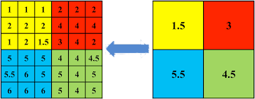
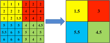
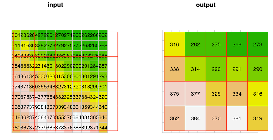
Raster Resampling - Methods
Nearest Neighbor Resampling
- The new raster pixels get the value from nearest pixel of the original raster to the center of the new pixel.
- Note that some of the values are lost this way (particularly in downsampling), since they were not passed on to the new raster
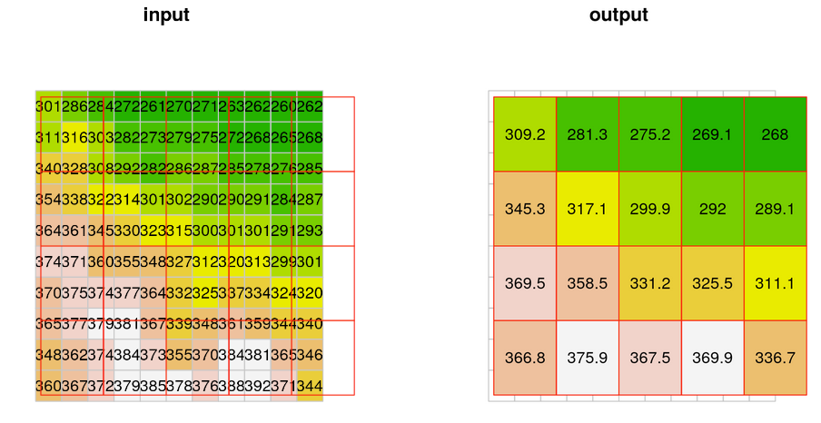
bilinear resampling
- Each new raster cell gets a weighted average of four nearest cells from the input, rather than just one
- Less loss of information
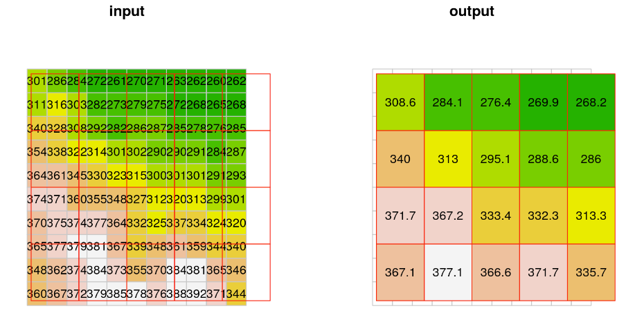
Average resampling
- Each new cell gets the (non-weighted) average of all overlapping input cells
Raster Resampling
There are two\(^*\) tools for resampling in QGIS
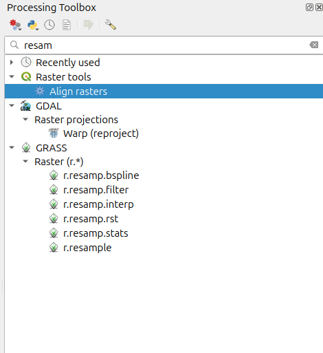
* Actually there are others, notably if Grass is installed its tools are also available.
| Feature | QGIS Align Rasters | GDAL Warp |
|---|---|---|
| Align to grid | ✅ Yes (to reference) | ✅ Yes (to round coords) |
| Resample | ✅ Yes | ✅ Yes |
| Match resolution | ✅ Yes | ⚠️ Only if specified |
| Match extent | ✅ Yes | ⚠️ Only if specified |
| Grid type | Reference raster | Integer/round coordinates |
- QGIS Align Rasters
- GDAL Warp is more flexible
- It can reproject
- It can clip to an extent
- It is a useful command line tool
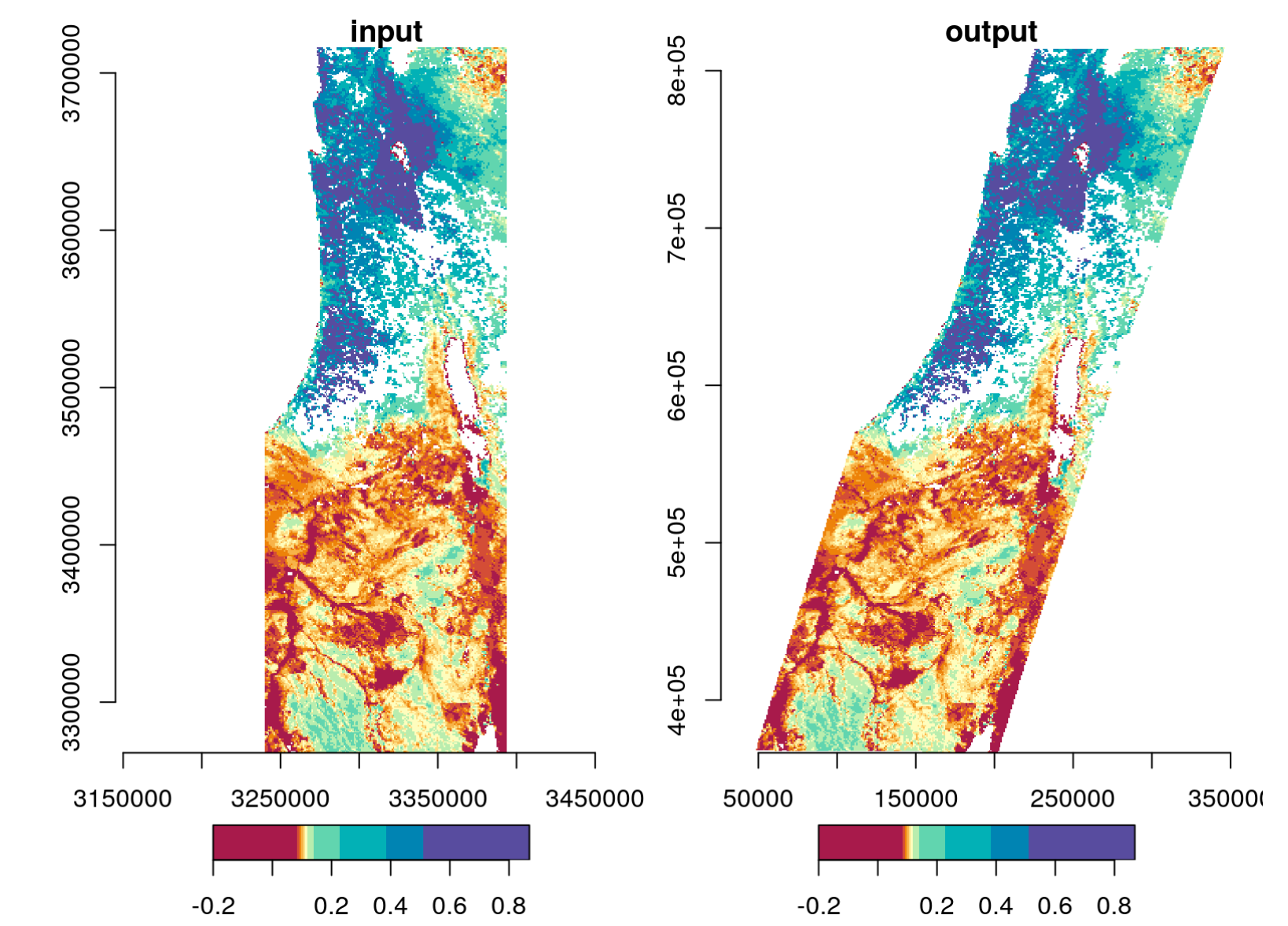
Raster Reprojection (Warping)
Just like vector data, we need to reproject rasters if we’re to do accurate analysis.
The goal is to realign the pixels, without changing their values.
The goal is to realign the pixels, without changing their values.
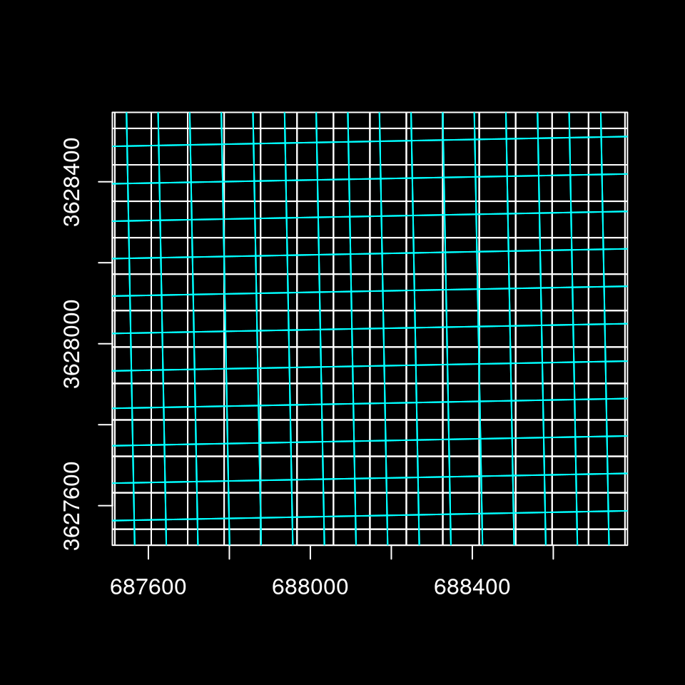
What happens in the reprojection can be thought of as a two-step process
- The pixel outlines are reprojected as if they were polygons
- This results in an irregular grid
- The grid is then resampled to form a regular grid
Raster Reprojection using GDAL Warp
Download
dw_2025.tif,dw_20218.tif, anddw_style.qmlfrom this linkIn QGIS open dw_2025.
- Look at the CRS
- Look at the resolution.
In the symbology tab, at the bottom left there is a style dropdown.
- select “Load Style…” use the browser to open the
dw_style.qmlfile from thedynamic_worldfolder - Apply
- select “Load Style…” use the browser to open the
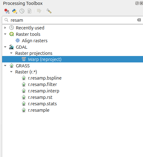
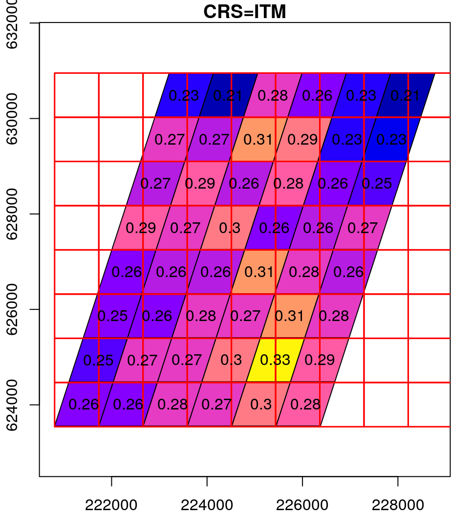
Reproject dw_2025 using GDAL Warp (Processing Toolbox: GDAL → Raster projection → Warp)
- Leave Source CRS blank (In “Input layer” you can see that the CRS is recognized)
- Set Target CRS to EPSG:6339
- Use average resampling
- Set ” Output file resolution in target georeferenced units” to 10
- What are the target georeferenced units?
- Leave the rest as defaults, including “[save to temporary Layer]”
Compare the results to the original. Do you see any problems?
Why is this margin of different land cover appearing?

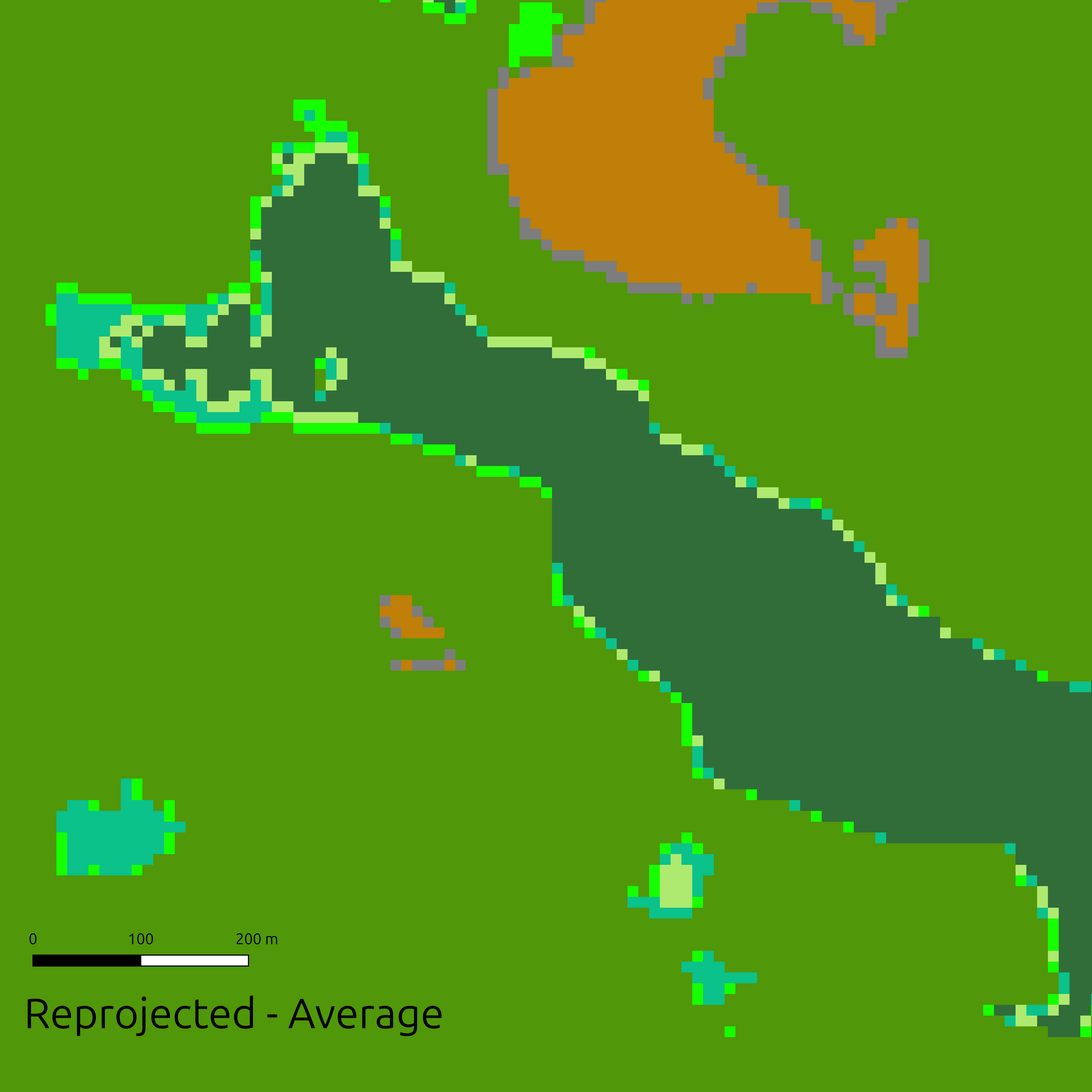
Try again, what resampling method should you use?
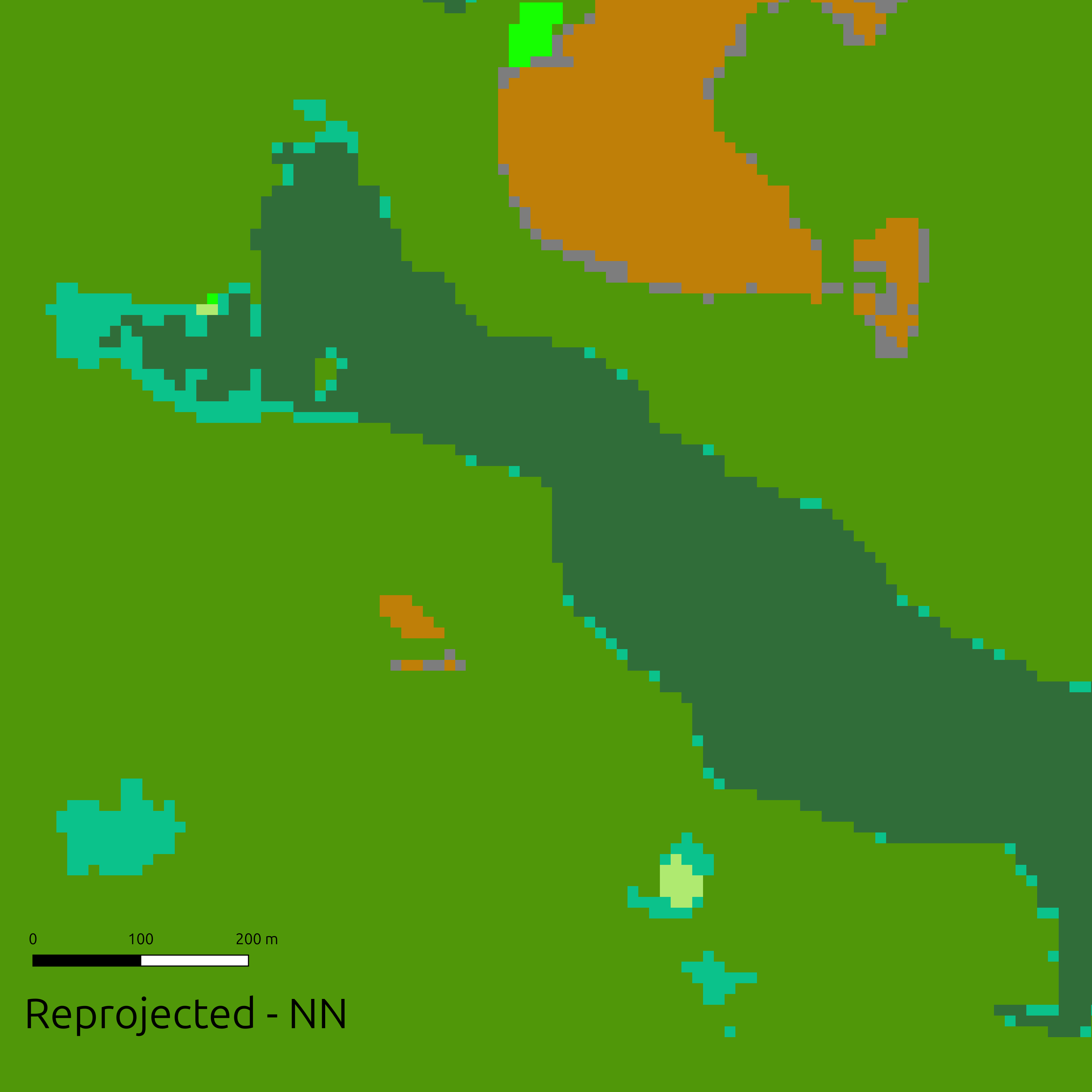
- Save the reprojected layer
dw_2025_6339.tif. - Reproject dw_2018 in the same way (save as
dw_2018_6339.tif)
- Use
Raster Tools → Align Rastersto aligndw_2018_6339.tifanddem_1m_6339.tifto dw_2025_6339 (use appropriate resample methods).
Now use the the Raster Calculator to find areas that were covered in trees in 2018, but not in 2025.
Can you figure out how to find areas that were covered in trees in 2018, but not in 2025 on a slope > 10% ?
Remote sensing
Remote sensing - Obtaining information about an object from a distance.
What is the most basic form of remote sensing you can think of?
Looking at something!
There are many different methods of remote sensing.
- Some ground based
- Some airborne
- Some satellite based
- Most remote sensing relies on electromagnetic radiation
Red band (0.63 - 0.69 µm)
Useful for:
- Detecting bare soil, buildings, pavement
- Chlorophyll absorption
Green band (0.52 - 0.6 µm)
Useful for:
- phenology / vegetation dynamics
- plant Health
- algal Blooms
Blue band (0.45 - 0.52 µm)
Useful for:
- water
- clouds
- snow
- aerosols
NIR band (0.77 - 0.9 µm)

Useful for:
- biomass
- vegetation detection
- boundary detection
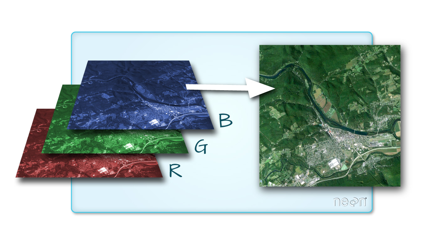
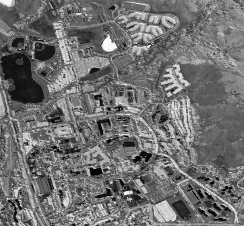
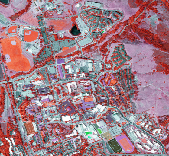
A “True Color” image used Red, Green and Blue
- Pixels in display contain 3 sub-pixels
- Each sub-pixels intensity is controlled by the intensity value in the image
- Intensity values are stored as 8-bit unsigned integers (
uint8)- 8 bits = \(2^{8}\) = 256 possible values
- Range: 0 to 255 (256 values total)
- Images are sometimes stored with higher precision, but displayed with 8 bits
(255, 0, 0)   = pure red
(0, 255, 0)   = pure green
(0, 0, 255)   = pure blue
(255, 255, 0) = yellow (red + green)
(0, 255, 255) = cyan (green + blue)
(255, 0, 255) = magenta (red + blue)
(255, 255, 255) = white (all combined)
(0, 0, 0)     = black (none)
Combining bands on different ways is often useful.
For example, False Color Image
- Near-Infrared to Red, Red to Green, and Green to Blue (NIR, G, R)
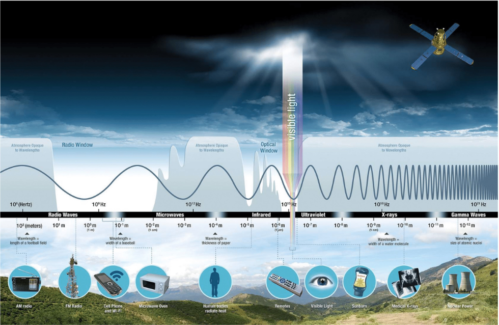
- Humans see only a small portion of the EM spectrum.
- Instruments on satellites capture more, but still only a small portion of the entire electromagnetic spectrum
Right: Reflectance of water, soil and vegetation in different wavelengths and Landsat TM channels.

Passive vs. Active
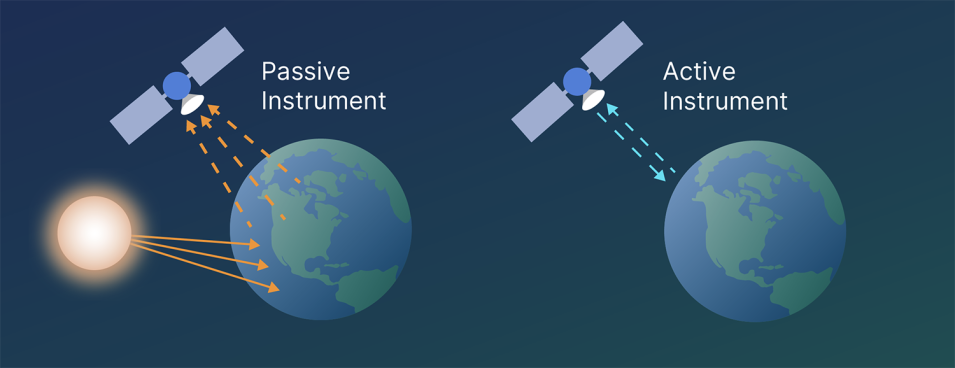
Image Source: NASA Earthdata
- The type of remote sensing we have been discussing so far is optical remote sensing.
- Optical remote sensing is a is passive
- Light from the sun bounces off of the earth and into the sensor (Eyeball, Camera, Radiometer)
- Radiometric sensing covers a wider spectral range, and may include active as well as passive techniques.
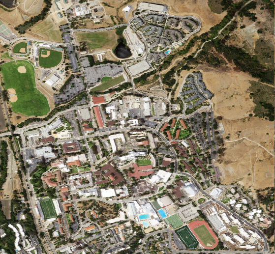
NAIP Imagery
National Agriculture Imagery Program (NAIP)
- High-resolution aerial imagery of the continental United States
- Collected during agricultural growing seasons
- Typically 4-band: Red, Green, Blue, Near-Infrared (NIR)
- 60 cm (or better) spatial resolution
- Updated on a 2-3 year cycle for each state
Learn more: USDA NAIP Program
Spectral Response Curves
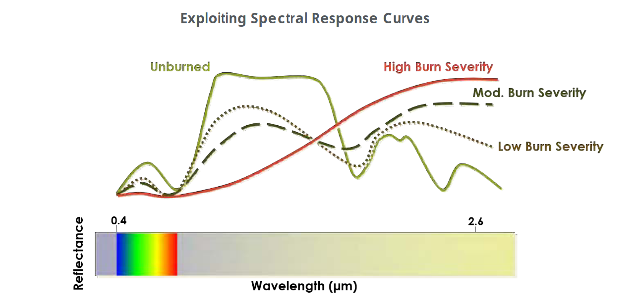
Image Source: SEOS
\[ \text{NBR} = \frac{\text{NIR} - \text{SWIR-2}}{\text{NIR} + \text{SWIR-2}} = \frac{B_8 - B_{12}}{B_8 + B_{12}} \]

NDVI
\((\text{NIR} - \text{Red}) / (\text{NIR} + \text{Red})\)
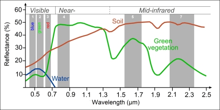
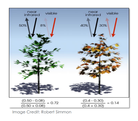
Image Source: NASA ARSET
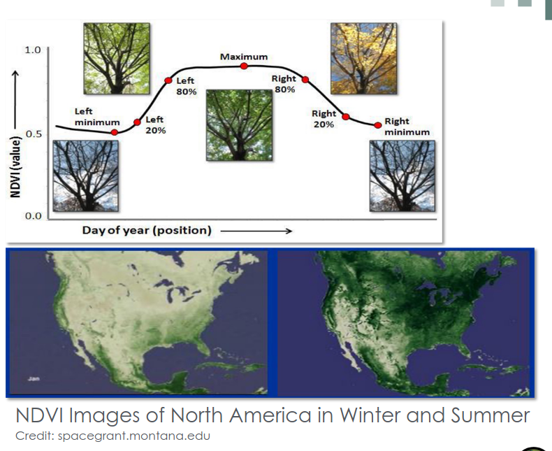
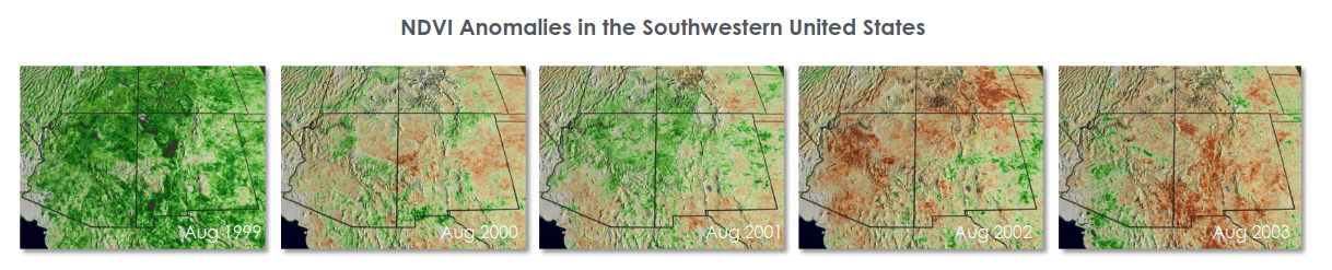
Image Source: NASA ARSET
Raster Resampling
Resampling is adjusting the pixel size or resolution of raster data in order to:
- Match resolutions - So multiple rasters will align1 for analyisis (e.g., NDVI and elevation)
- Downsample - Reduce resolution for faster processing
- Upsample - Increase resolution for finer analyses (though it won’t create new information)
Raster Resampling - Methods
Nearest Neighbor Resampling
- The new raster pixels get the value from nearest pixel of the original raster to the center of the new pixel.
- Note that some of the values are lost this way (particularly in downsampling), since they were not passed on to the new raster
bilinear resampling
- Each new raster cell gets a weighted average of four nearest cells from the input, rather than just one
- Less loss of information
Average resampling
- Each new cell gets the (non-weighted) average of all overlapping input cells
Raster Resampling
There are two\(^*\) tools for resampling in QGIS
* Actually there are others, notably if Grass is installed its tools are also available.
| Feature | QGIS Align Rasters | GDAL Warp |
|---|---|---|
| Align to grid | ✅ Yes (to reference) | ✅ Yes (to round coords) |
| Resample | ✅ Yes | ✅ Yes |
| Match resolution | ✅ Yes | ⚠️ Only if specified |
| Match extent | ✅ Yes | ⚠️ Only if specified |
| Grid type | Reference raster | Integer/round coordinates |
- QGIS Align Rasters
- GDAL Warp is more flexible
- It can reproject
- It can clip to an extent
- It is a useful command line tool
Raster Reprojection (Warping)
Just like vector data, we need to reproject rasters if we’re to do accurate analysis.
The goal is to realign the pixels, without changing their values.
The goal is to realign the pixels, without changing their values.
What happens in the reprojection can be thought of as a two-step process
- The pixel outlines are reprojected as if they were polygons
- This results in an irregular grid
- The grid is then resampled to form a regular grid
Raster Reprojection using GDAL Warp
Download dw_2025.tif and dw_20218.tif as well as dw_style.qmlhttps://cpslo-my.sharepoint.com/:u:/g/personal/mthuggin_calpoly_edu/EXMEE6bR85VMkOPotG9dk6sBbr2JQx2QNFtsR9-0OAIQfg?e=aa09WA
In QGIS open dw_2025.
- Look at the CRS
- Look at the resolution.
In the symbology tab, at the bottom left there is a style dropdown.
- select “Load Style…” use the browser to open the
dw_style.qmlfile from thedynamic_worldfolder - Apply
- select “Load Style…” use the browser to open the
Reproject dw_2025 using GDAL Warp (Processing Toolbox: GDAL → Raster projection → Warp)
- Leave Source CRS blank (In “Input layer” you can see that the CRS is recognized)
- Set Target CRS to EPSG:6339
- Use average resampling
- Set ” Output file resolution in target georeferenced units” to 10
- What are the target georeferenced units?
- Leave the rest as defaults, including “[save to temporary Layer]”
Compare the results to the original. Do you see any problems?
Why is this margin of different land cover appearing?
Try again, what resampling method should you use?
- Save the reprojected layer
dw_2025_6339.tif. - Reproject dw_2018 in the same way (save as
dw_2018_6339.tif)
- Use
Raster Tools → Align Rastersto aligndw_2018_6339.tifanddem_1m_6339.tifto dw_2025_6339 (use appropriate resample methods).
- Now use the the Raster Calculator to Find areas that were covered in trees in 2018, but not in 2025.
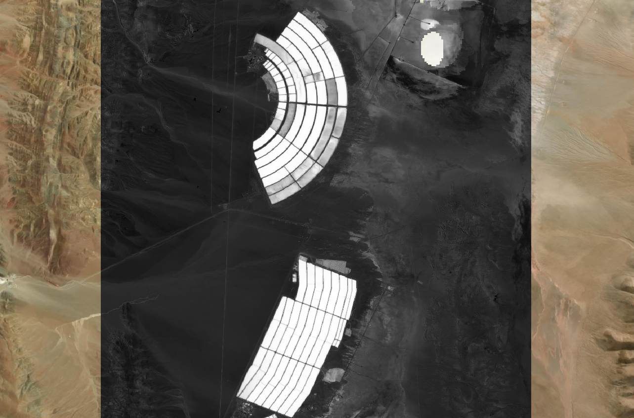
What kind of information is needed to segment this image?
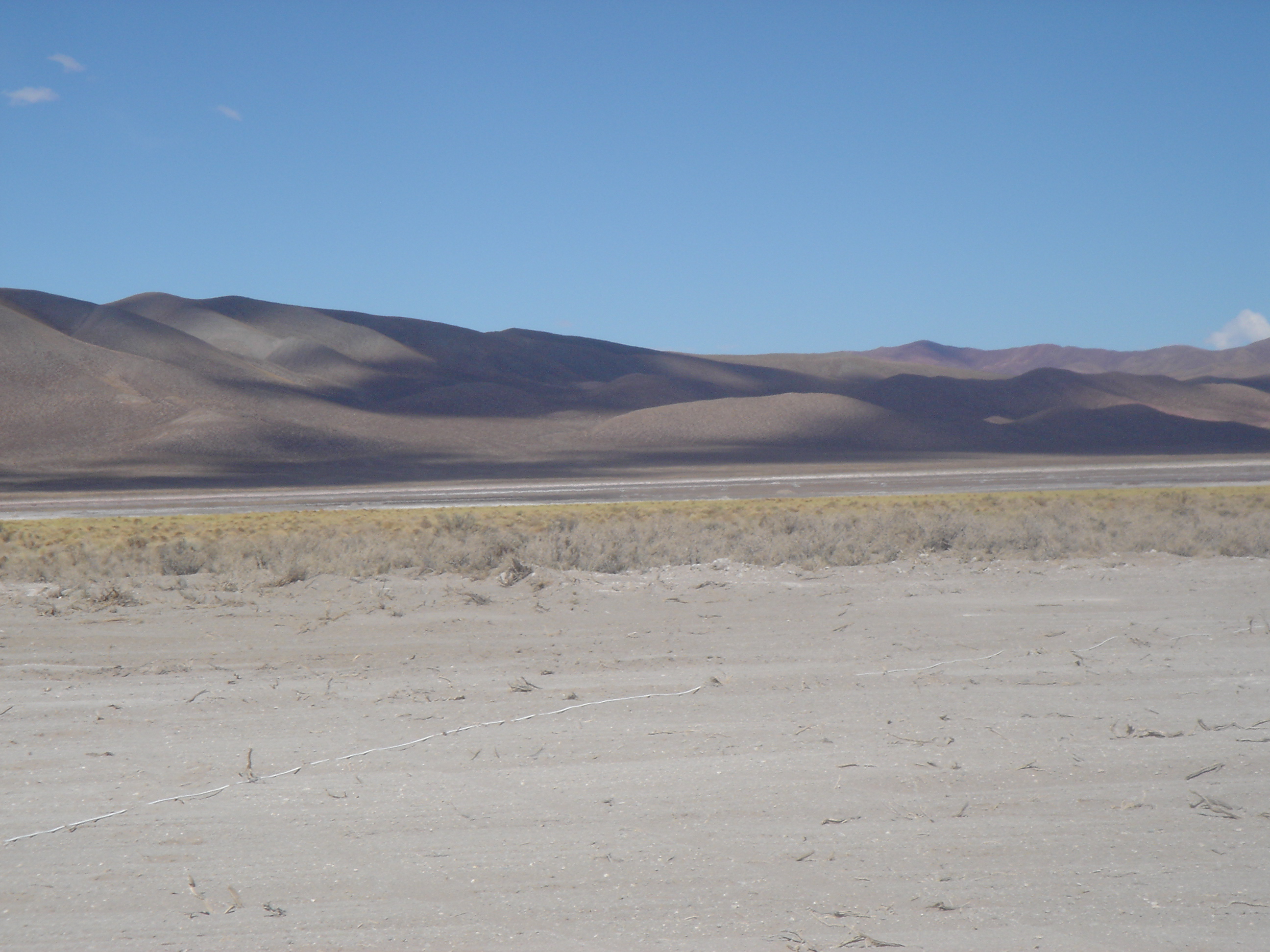
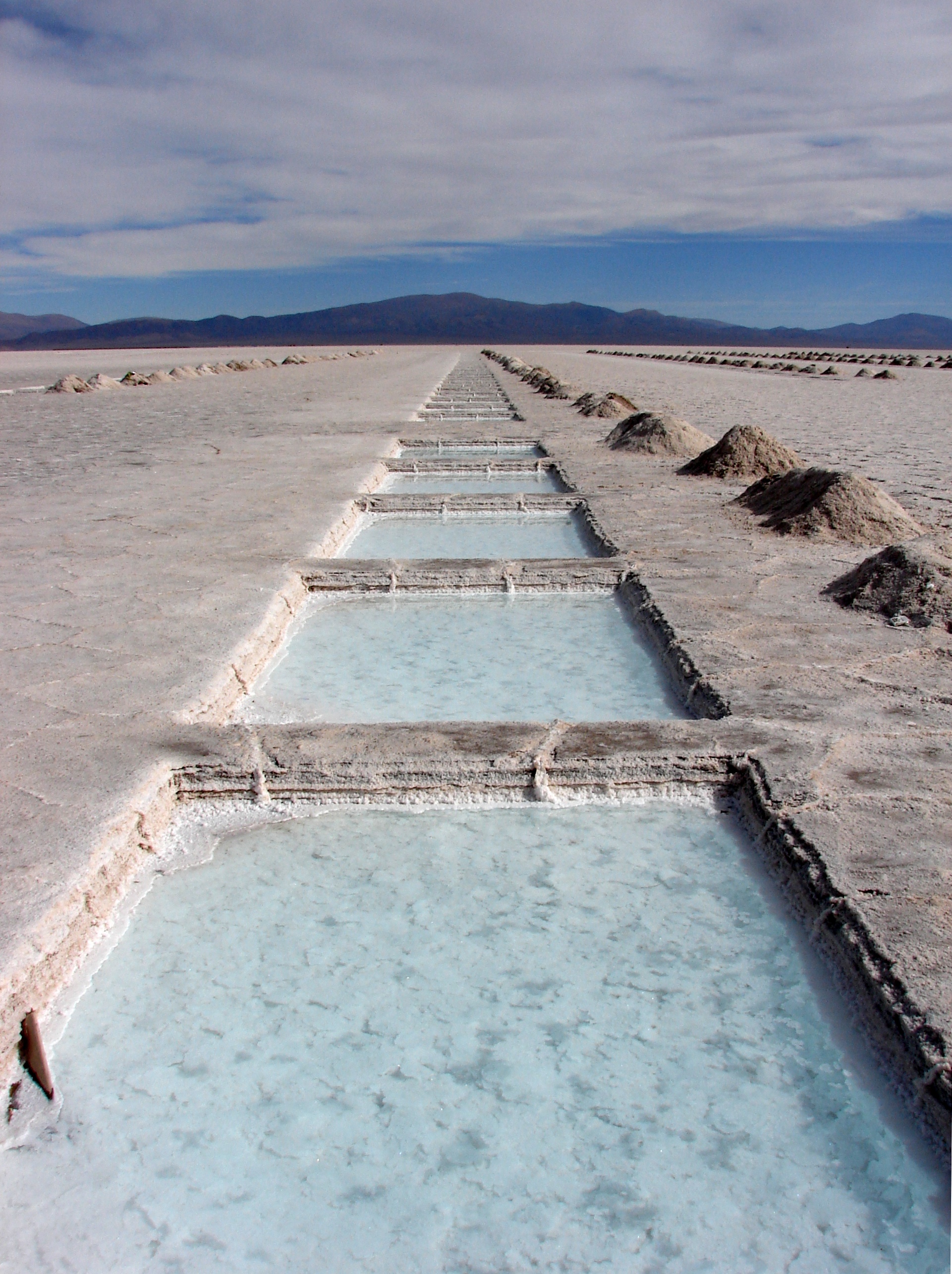
In Lab 11 you you are asked to segment the image to find lithium brine evaporation ponds near Susques Argentina.
If you have looked at the images over a basemap, or searched for Susques on the internet, you may have learned that it is in the Atacama desert.
The Atacama, being a desert, is quite dry (actually, it is one of the driest places on Earth!).
If you happened to google lithium evaporation pond, you probably know that they are used to evaporate lithium brine in order to extract lithium salts.
Given this information, one would expect these lithium ponds to be wetter than their surroundings.

Segmentation using Raster Calculator
In simple cases one can use the raster calculator.
- Calculate you index.
- Calculate you index.
- Use Raster calculator to segment values above a threshold
Installing Orfeo Toolbox
In this class we will use Orfeo Toolbox, an open source remote sensing project, but there are many other options.
Go to the Orfeo Toolbox download page and click the Download OTB 9.x.x.x button.
Or if that link is broken use this copy.
Extract the file and move the resulting folder to your home directory.
Install the Orfeo Toolbox Provider pluggin.
Install the Orfeo Toolbox Provider pluggin.
Open processing toolbox and click the settings icon
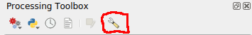
Open processing toolbox and click the settings icon
- Click the Processing tab on the left
- Click the OTB dropdown
- Check the activate box, if it exists
- Select the OTB application folder by browsing to
~/OTB.x.x.x/lib/otb/applicationsand click select folder (x.x.x is just a place holder for whatever version you have) - Set OTB folder to
~/OTB.x.x.x
You can watch this painfully slow video if you are having trouble.
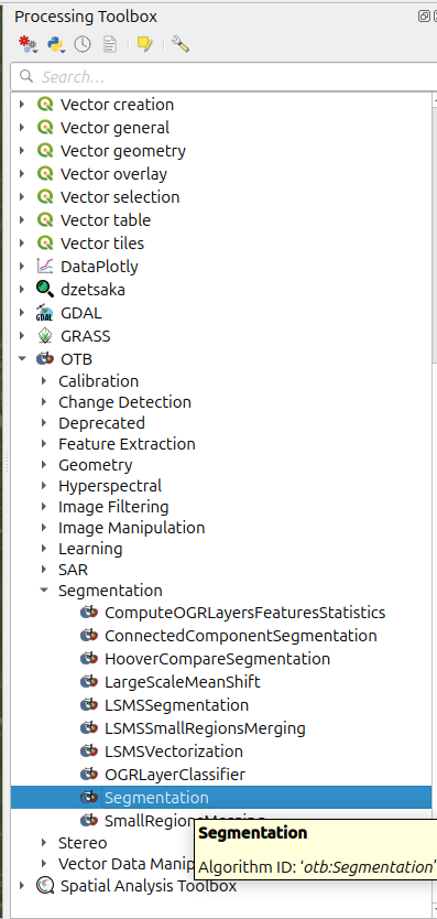
Segmentation
| Band | Common name | Central wavelength (nm) | Resolution (m) | |
|---|---|---|---|---|
| B1 | Coastal aerosol | 443 | 60 | |
| B2 | Blue | 490 | 10 | |
| B3 | Green | 560 | 10 | |
| B4 | Red | 665 | 10 | |
| B5 | Red Edge 1 | 705 | 20 | |
| B6 | Red Edge 2 | 740 | 20 | |
| B7 | Red Edge 3 | 783 | 20 | |
| B8 | NIR | 842 | 10 | |
| B8A | Narrow NIR | 865 | 20 | |
| B9 | Water vapor | 945 | 60 | |
| B10 | Cirrus | 1375 | 60 | |
| B11 | SWIR 1 | 1610 | 20 | |
| B12 | SWIR 2 | 2190 | 20 |
- Using Raster Calculator, extract Band 4 from the image, (can be scratch layer, rename it NIR)
- Run Zonal Statistics using the segments and the NIR raster, calculate mean
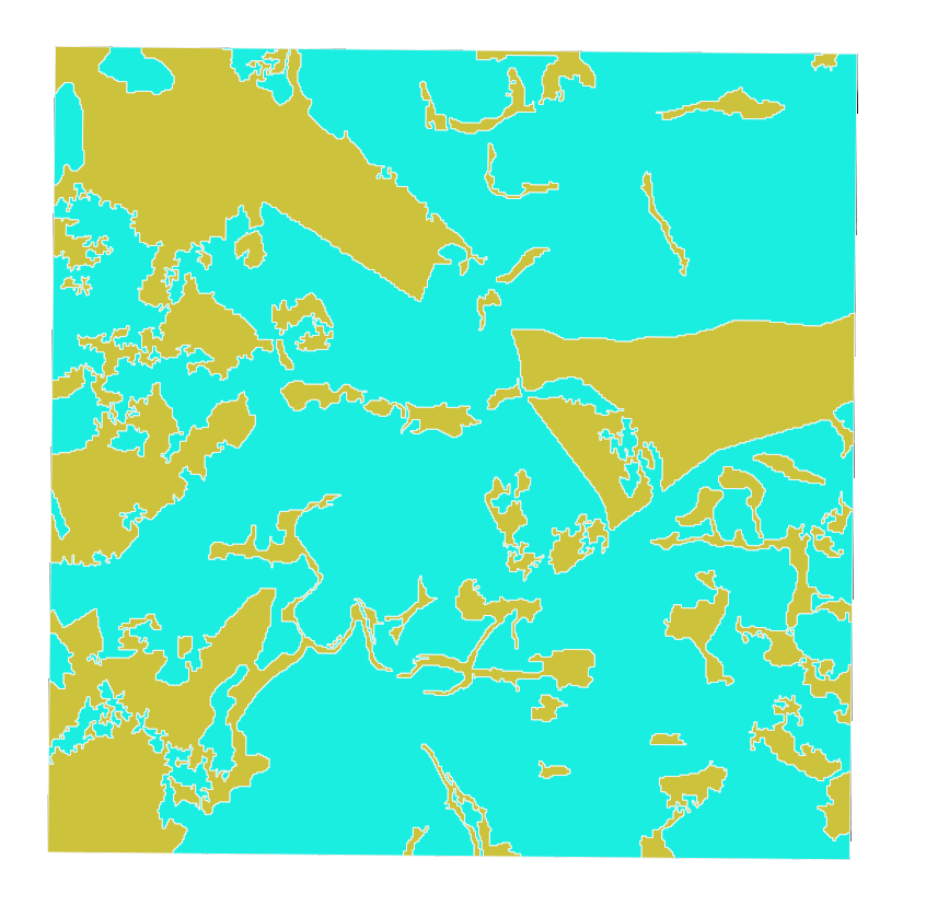
- In the geoprocessing toolbox, find K-means clustering (ABC) under Attribute based clustering
- Run with 2 clusters, and class as the value “Fields to use for clustering”
- Dissolve the output (Clusterd Layer) based on on class
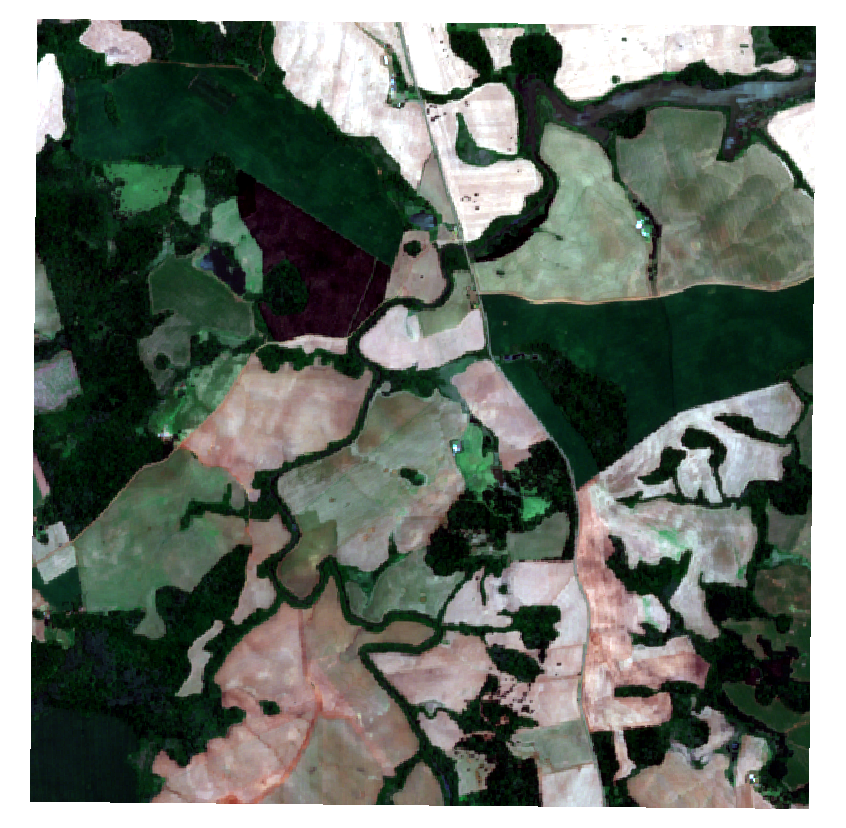
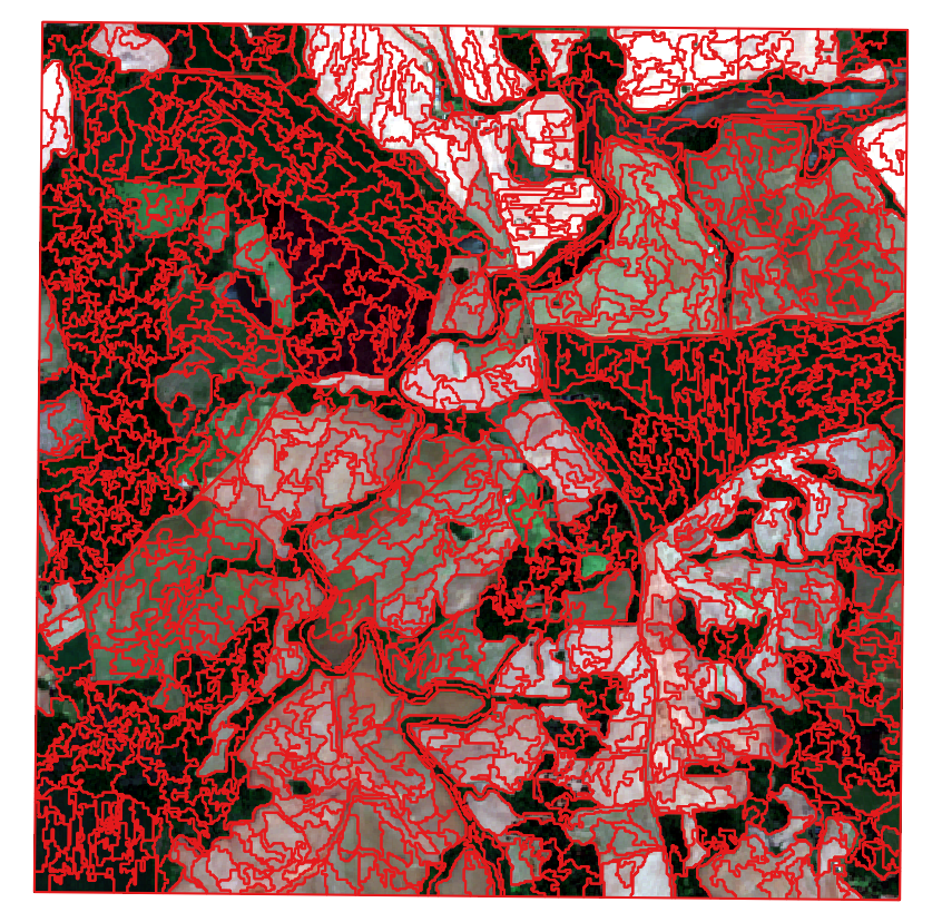
This image contains Sentinel2 bands 4, 3, 2 and 8.
- Go to Processing Toolbox > OTB > Segmentation > Segmentation
- You can run the algorithm with default settings, except you need to specify an output file (use a .shp file as output, Orfeo complains about geojson for some reason.)
- You should end up with something like this (after you adjust the symbology)
Population v. Sample
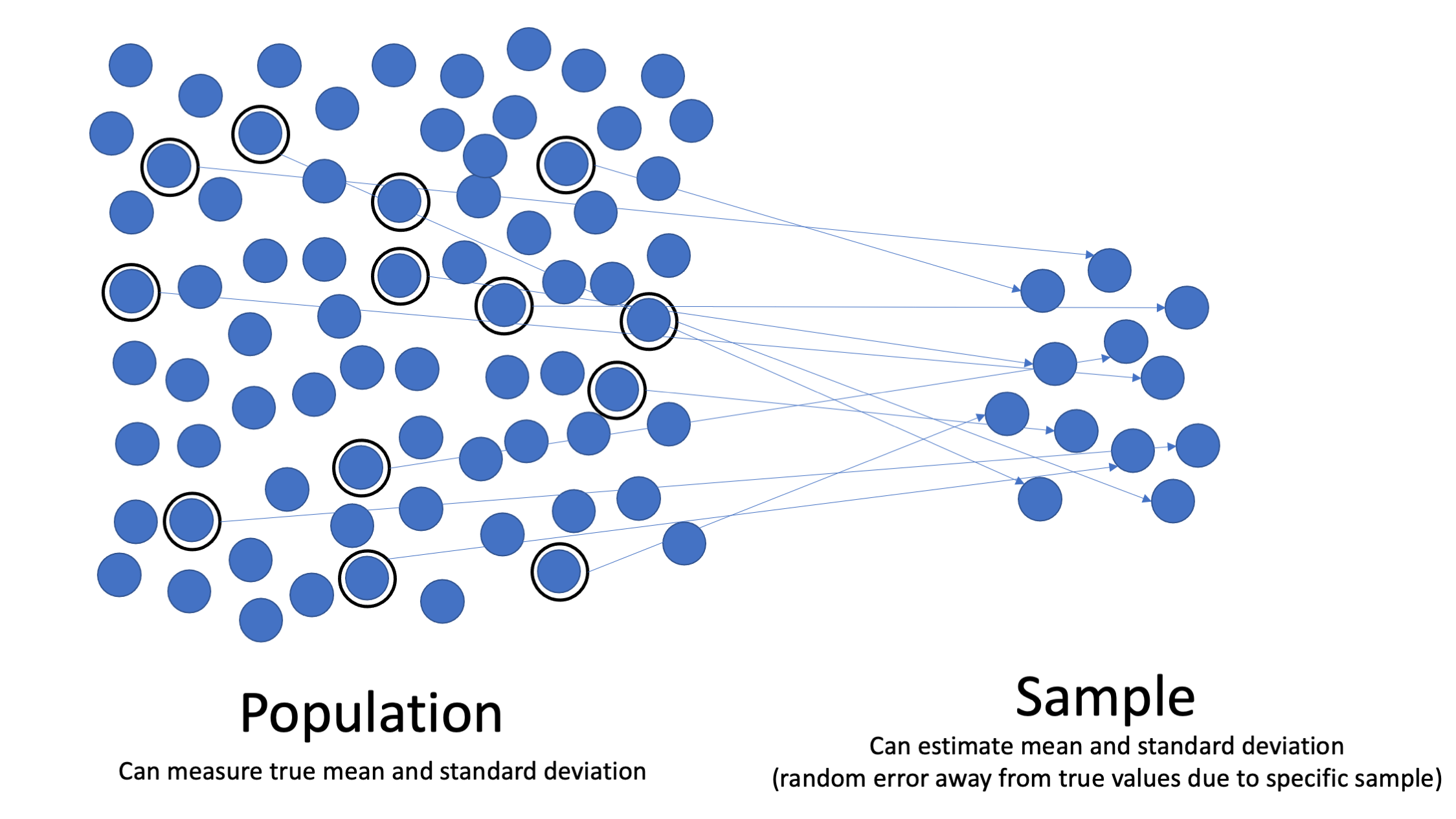
Image Source: Wikimedia
Population Variance (Parameter)
\(\sigma^{2} = \frac{\sum (x - \mu)^{2}}{N} = ?\)
Sample Variance, unbiased estimator (statistic)
\(s^{2} = \frac{\sum (x - \bar{x})^{2}}{n - 1} = 0.038\)
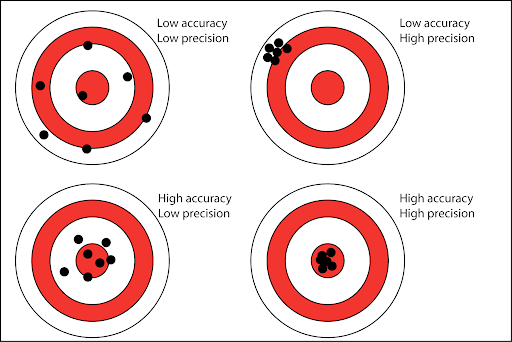
Precision v. Accuracy
- Higher spatial resolution does not inherently make the data more accurate - though higher resolution data can be described as more precise
- Spatial resolution can affect the accuracy of analysis performed with the raster data,
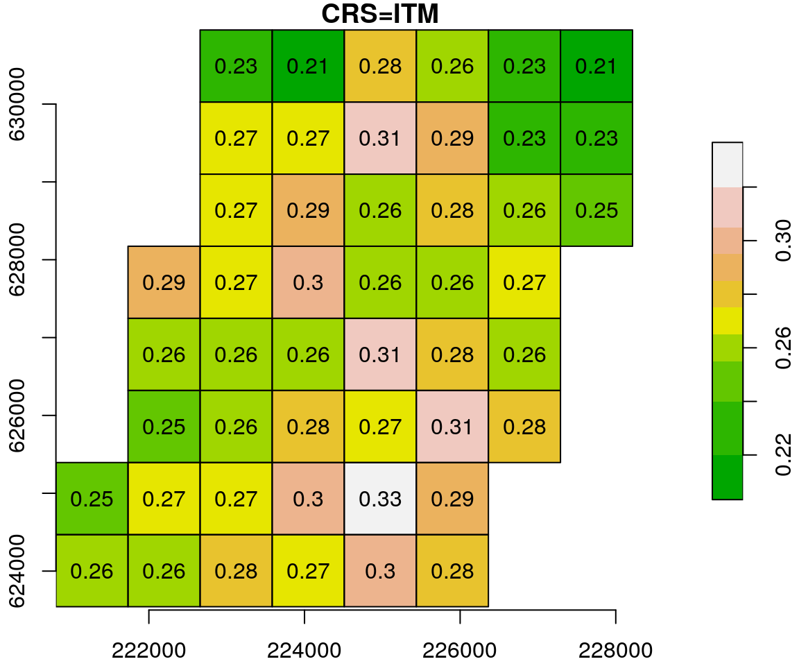
Extracting Raster Values
Sometimes we would like to know the raster values at points, along a line, or within a polygon.
Extracting Raster Values by Point
- Consider the elevation data and rain gauge locations at Swanton Ranch.
- What if we want to know the elevation of all rain gauges represented points?
Processing Toolbox → Sample raster values
- Input layer = points
- Raster layer = elevation
- Output column prefix = “Elevation_”
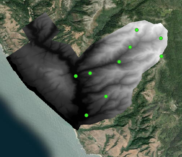
Now use the Field Calculator to calculate the mean and standard deviation!
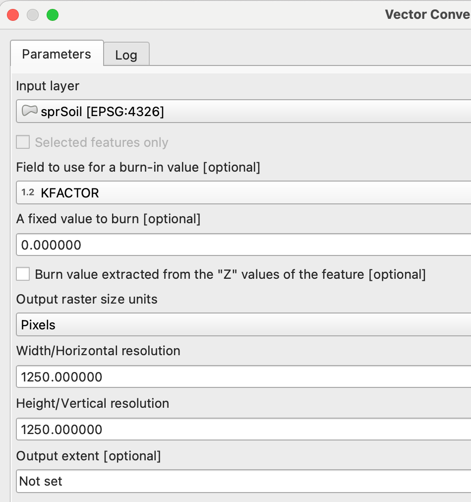
Converting Vector Data to Raster
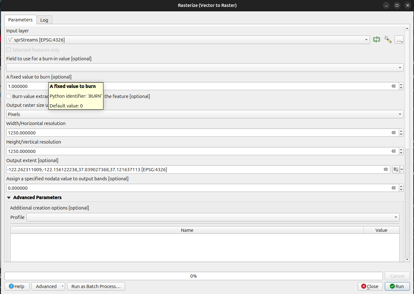
Input Later: sprStreams Fixed Value to burn: 1 Output Raster Size units: Pixels Width/Horizontal Resolution: 1250 Height/Vertical Resolution: 1250 Output Extent: Calculate from layer (sprStreams)
Raster → Contours
Raster → Extraction → Contours
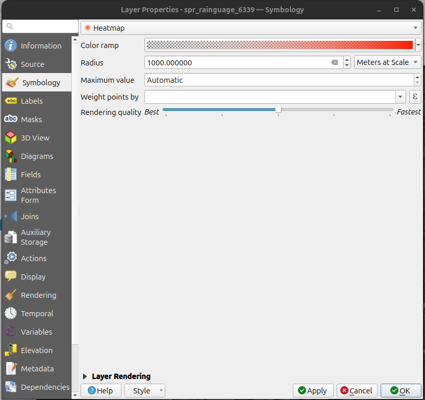
Heatmaps
Rasterize by Attribute - Symbolize by Value
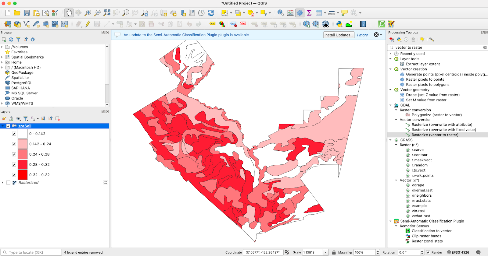
Raster>Conversion>Rasterize(Vector to Raster)- Layer = sprSoil
- Field = KFACTOR
- Output raster size units = Pixels
- Horizontal / Vertical Resolution = 1250
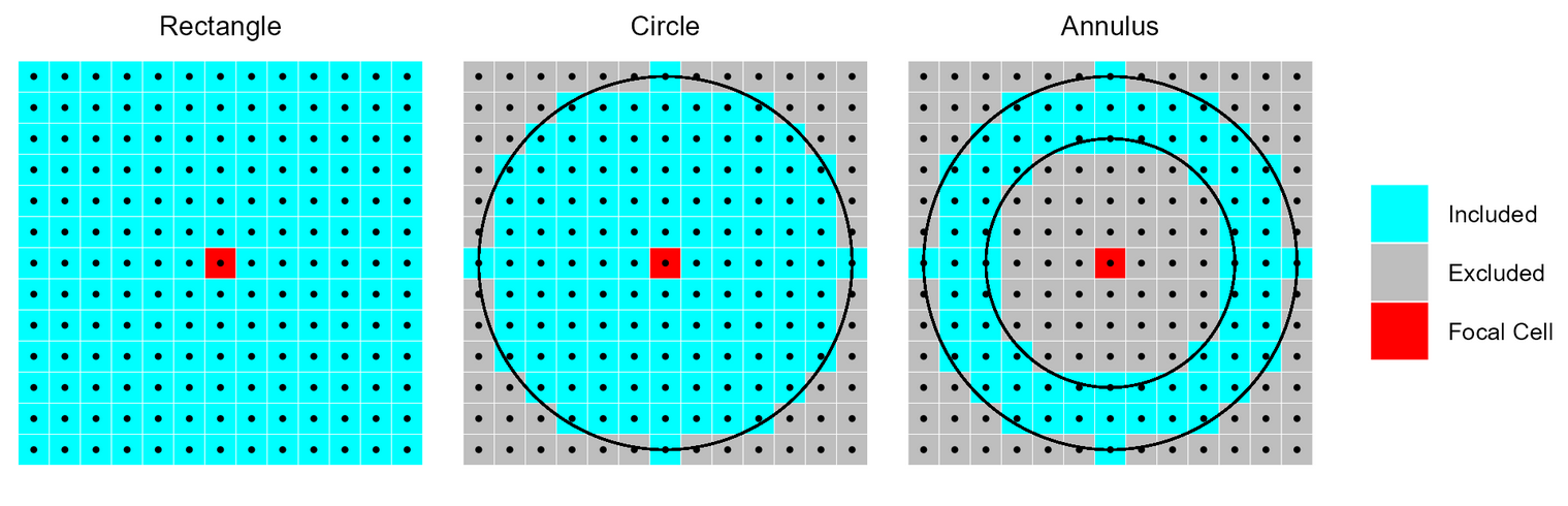
Kernels & Weights
- Kernels are matrices of weights used to combine neighbor values into a new pixel.
- Weight patterns emphasize directions, distances, or specific neighbors.
Mean (a.k.a. Low-Pass) Filter
- Averages the values within the neighborhood, producing a smoothed surface.
- Dampens high-frequency variation
- Useful for removing noise from continuous surfaces (elevation, temperature, etc.).
Median Filter
- Replaces the center cell with the median of neighborhood values.
- Preserves edges better than mean smoothing while removing salt-and-pepper noise.
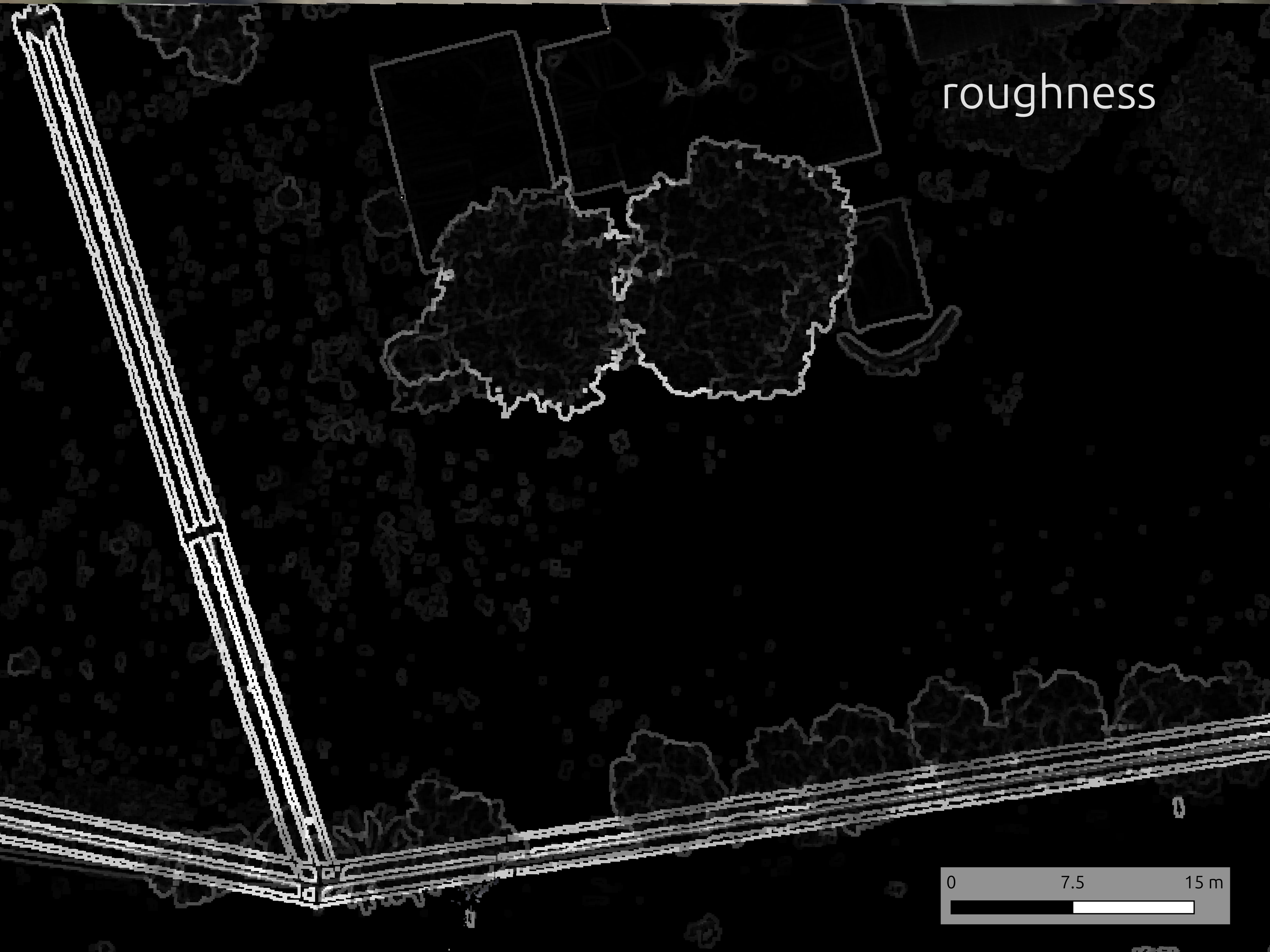
Roughness Filters
- Quantify variability inside the neighborhood (e.g., range, standard deviation).
- Capture terrain ruggedness, habitat heterogeneity, or surface texture.
- Sensitive to window size: smaller windows detect micro-relief; larger windows show broader roughness zones.
Raster>Analysis>Roughnesscomputes elevation range within a kernel in QGIS
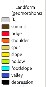
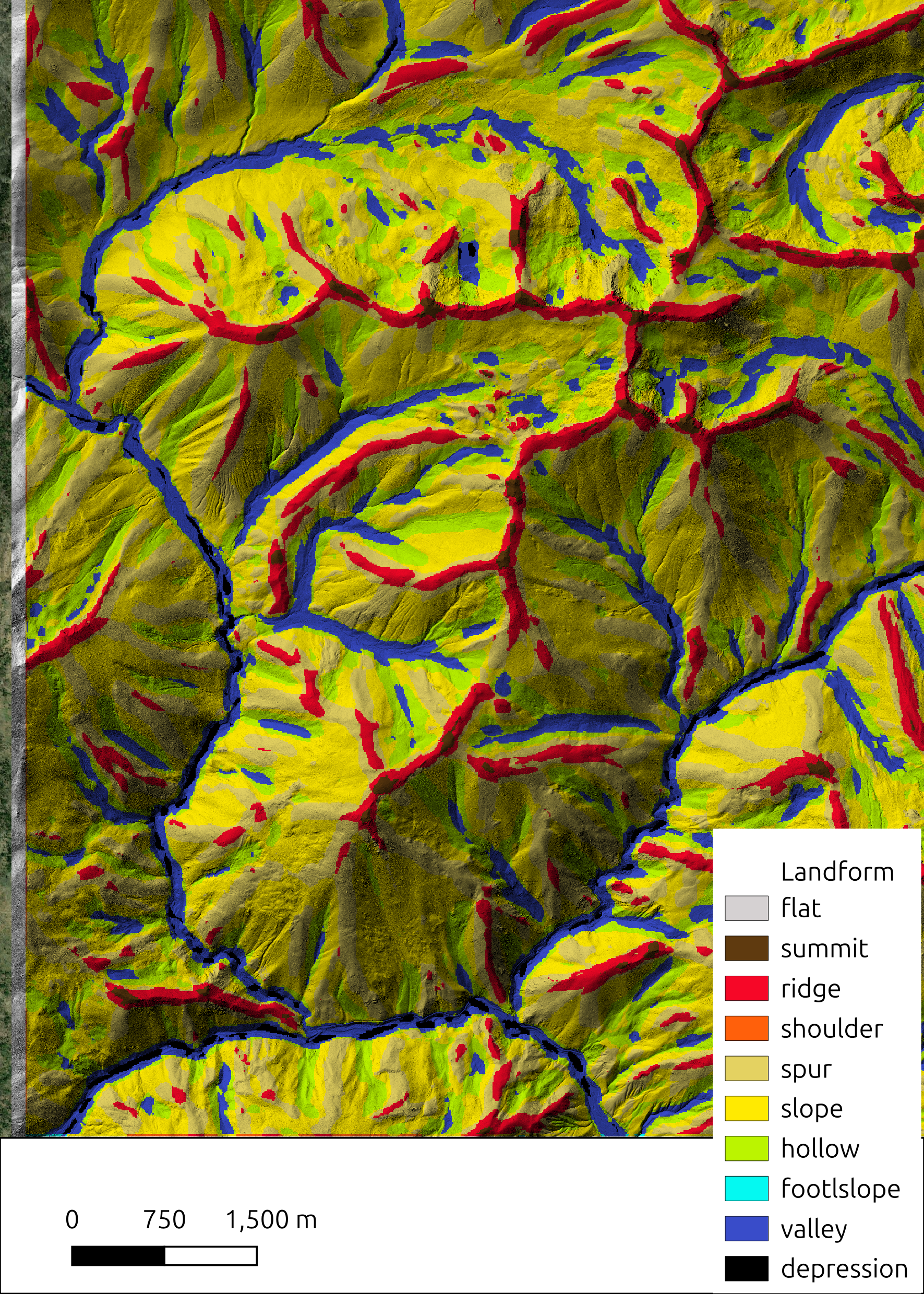
TPI & Geomorphons
- Topographic Position Index (TPI) compares a cell to the mean elevation of its neighbors.
- Positive TPI marks ridges; negative TPI highlights valleys—kernel size sets the landform scale.
- Geomorphons classify landforms using multi-directional TPI, revealing patterns such as spurs, hollows, and plains.
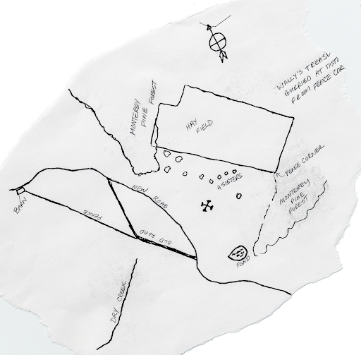
Example: Swanton Ranch Treasure Map
Download the Swanton Ranch treasure_map.tif. Put it someplace sensible.
Normal TIFs, No Georeferencing
This is just a regular tif, but we want to use it in a GIS program
Tutorial: Geoferencing the Treasure Map
- Open QGIS
- Open Georeferncer (
Layer>Georeferencer) - Open the raster (this button
![]() )
) - Select
treasure_map.tif![]()
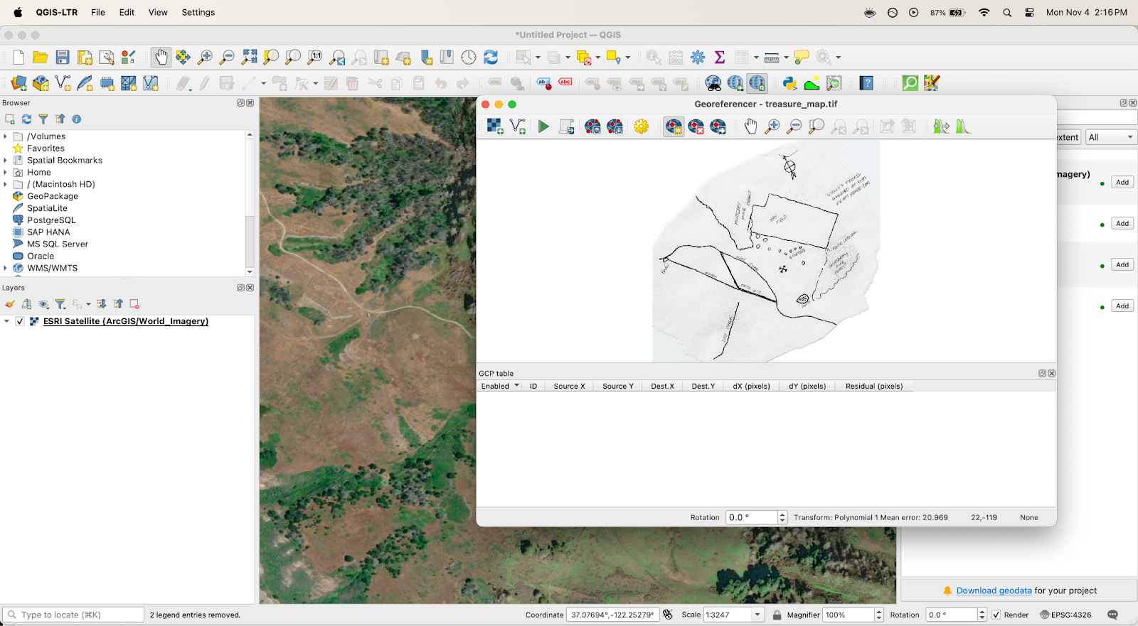
- Open Transformation Settings
- Select
Polynomial 1forTransformation Type - Set output file
- Click ok
![]()
![]()
Can anyone find where (in Swanton) our treasure map might correspond to?
What geographic features are helpful for identifying?
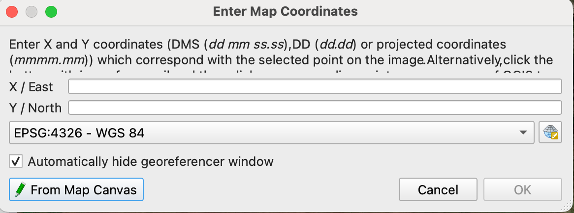
- Once you find the place:
- Add GCPs
- Click a point on the image
- The
Enter Map Coordinatesbox should pop up - Select the
From Map Canvasbutton - Click point
- Click ok
- Repeat 4x
![]()
Georeferencer dialogue should look like this:
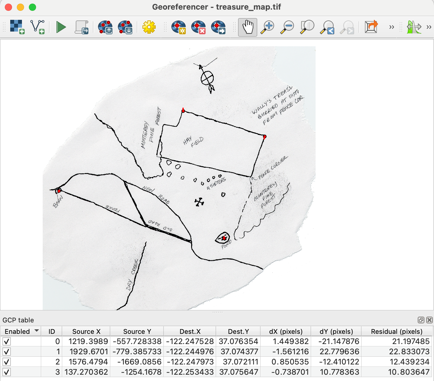
Click Run
![]()
Inspect the result - turn on transparency
Mini Lab: Exploring ArcGIS Pro
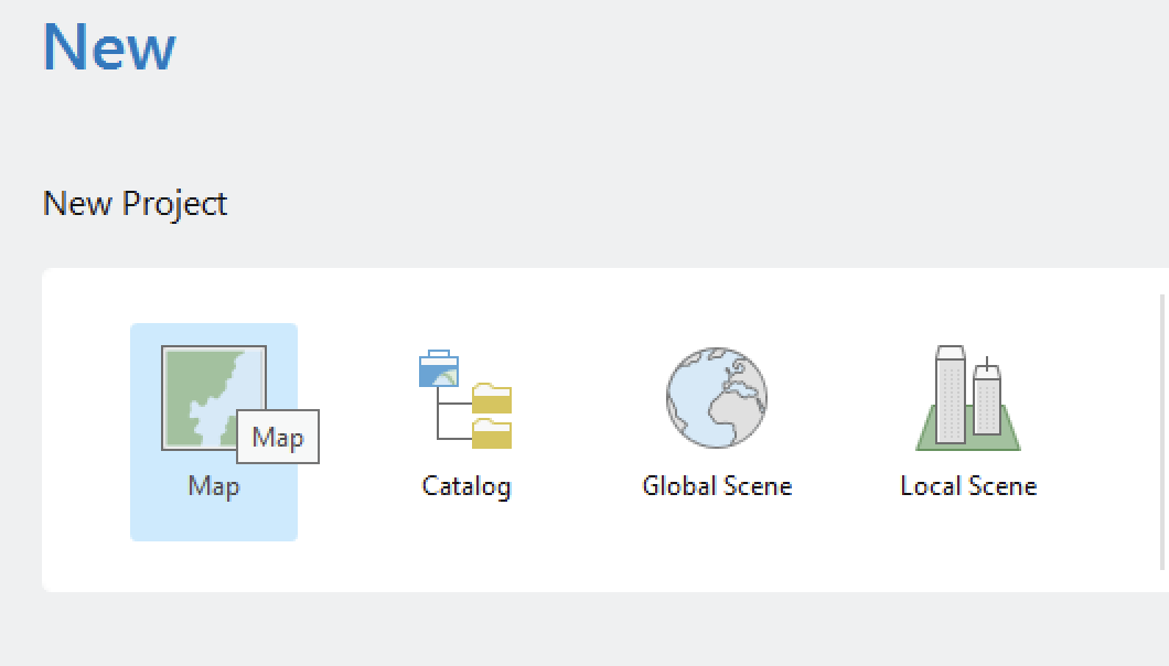
Opening ArcGIS Pro
- Use Cal Poly SSO
- Click on Map
- Make sure you know where the project is saved!
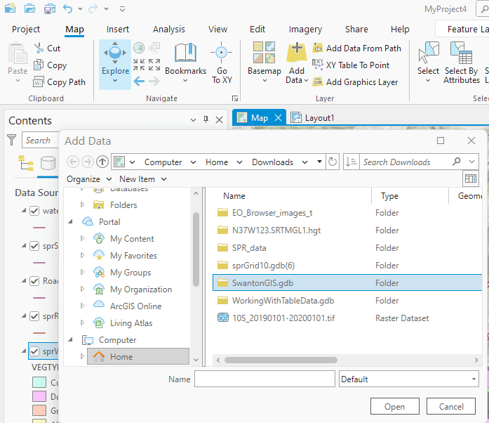
Adding data
- Download SwantonGIS.gdb.zip (new file type!)
- Unzip the file, save the whole .gdb to a new lab folder
- Add the data to your ArcGIS project
- Map > Add Data > Navigate to the GDB
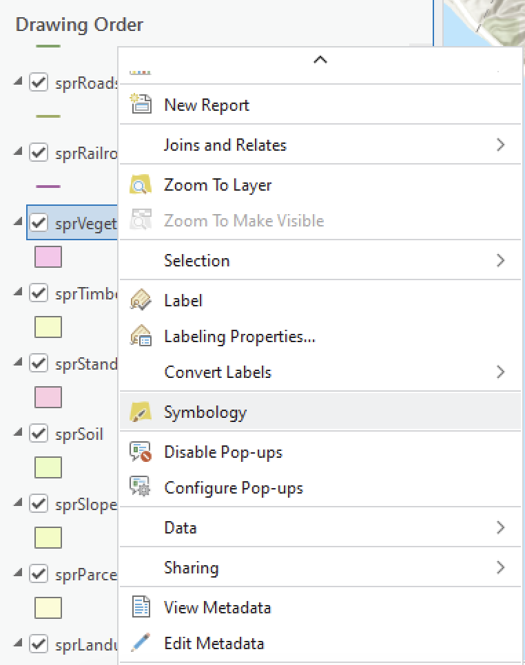
Adjusting symbology
- Right click on sprVegetation
- Go to Symbology
- Primary Symbology > Unique Values
- Field: VEGTYPE1
- Try out a few symbologies for numerical data (use a different layer)
- Symbology > Graduated Colors > KFACTOR
- Symbology > Graduated Symbols > Depth
- Symbology > Proportional Symbols > Slopemax
Making a Map in ArcGIS Pro
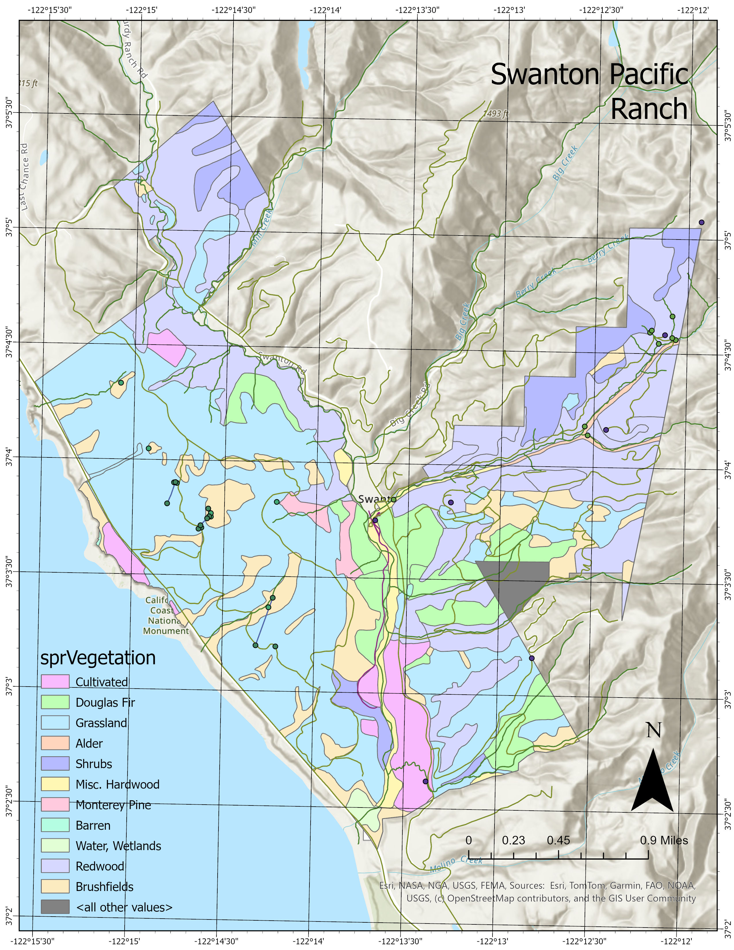
- Insert > New Layout > 8.5x11 Letter
- Insert > Map Frame
- Right click on Map Frame > Activate
- Right click on the sprVegetation layer in the layout tab > Zoom to Layer
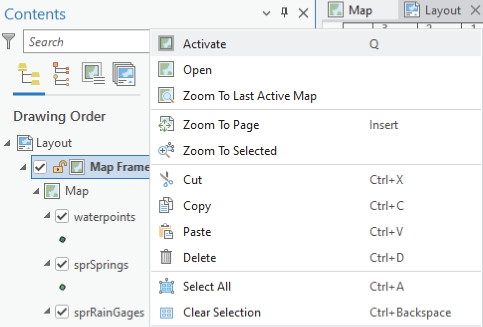
- When you’re satisfied, Layout > Close Activation
Other things we can add:
- Legend, scale bar, north arrow
- Latitude / longitude coordinates with
Grid - Also worth looking through the options under
Dynamic text