A Quick Lesson in Multi-band Rasters Using NAIP
In this exercise you will explore some visualizations and calculate simple spectral indices using NAIP imagery, as well as getting practice performing spatial overlays and merging vectors.
Create a document, answer the questions and include the requested figures. Submit the document as pdf on Canvas.
Questions will be included in this format, with a sidebar and in grey, throughout the exercise.
Data and directory structure
First we will need the data. Download the vector file of fire perimeters and 2022 NAIP (see Tip 1 for information about NAIP ) image below. The NAIP image may take a while, but should be done by the time you need it.
The fire perimeters data is a subset of polygons from California Historical Fire Perimeters dataset from California Open Data Portal.
The National Agriculture Imagery Program (NAIP) acquires aerial imagery during the agricultural growing seasons in the United States. It is generally made available to governmental agencies and the public within a year of acquisition.
- High-resolution aerial imagery of the continental United States
- Collected during agricultural growing seasons
- Typically 4-band: Red, Green, Blue, Near-Infrared (NIR)
- 60 cm (or better) spatial resolution
- Updated on a 2-3 year cycle for each state
Create a working directory, called lab_10, for this lab in you nr218 Folder. Create a data folder and put the downloaded data inside. Also create a docs directory and an img directory in the lab directory. You will store your submission document in docs, and any images you create in img.
Open QGIS, start a new project, and save it in the lab_10 folder as lab10_your_name.qgz (use your actual name)
You should then have something like this.
lab_10/
├── lab10_your_name.qgz
├── data/
│   ├── subset_of_cal_hist_fires.geojson
│   └── naip_2022.tif
└── docs/
└── img/
Your submission document, as well as any images
Data Preparation
- Open the fire perimeters dataset in QGIS.
fires_in_AOI
Extract the perimeter of the Coffee Fire (
FIRE_NAMEisCOFFEE). There are a few ways you can do this, your choice. Name the resulting layerCoffee(and save a file).Reduce the fire perimeter layer,
subset_of_cal_hist_fires, by selecting only fires that have happened since 2014 (Hint: extract by attribute). i.e.YEAR_ > 2013. Name the resulting layerscratch_1.Now extract all of the polygons which overlap the
Coffee(Hint: “select by location”). Name the result,scratch_2.Use the “Extract layer extent” tool to get a polygon of the extent of the Coffee fire. Name the result
extent.Buffer “extent” by 1000 m, use mitered joint style. (try it with default joint style too, what is the difference). name the buffered layer, our area of interest,
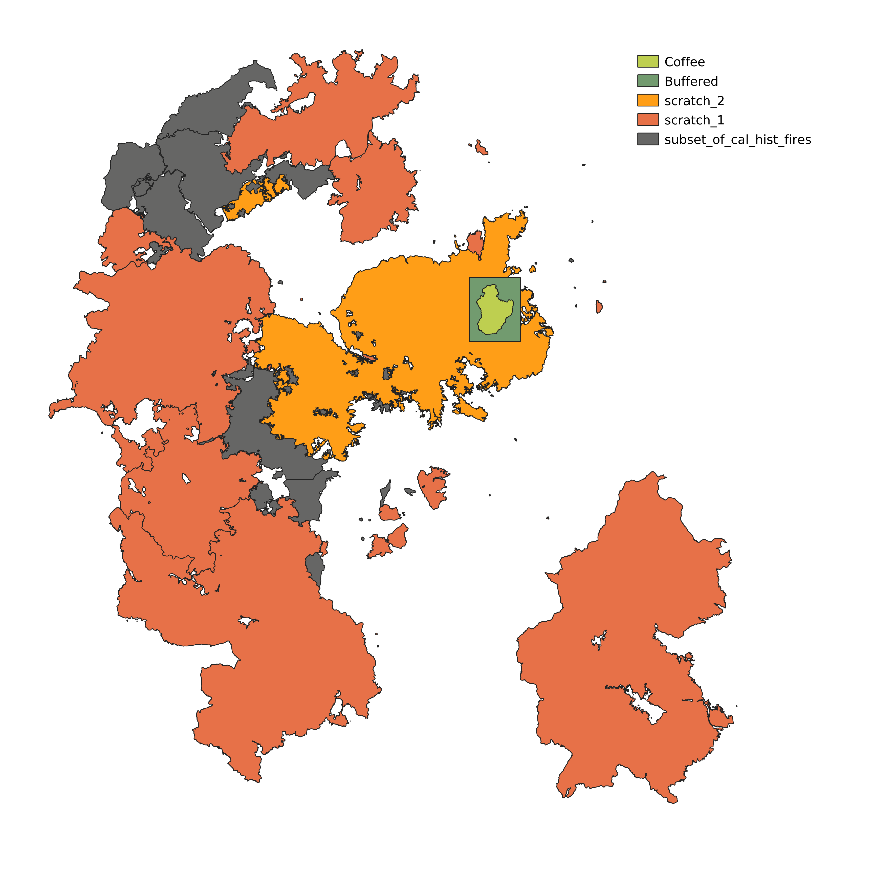
AOI. Figure 1 shows the layers that should have been created at this point (AOI is still calledBufferedin the image).Clip
scratch_2by the AOI. Save the results asfires_in_AOI.When you are satisfied that
fires_in_AOIturned out correctly you can deletescratch_1,scratch_2, andextent.
- Open
naip_2022. If you have a basemap on, turn it off so that the NAIP imagery is over a white background. Notice that the image looks very pale. Open the Layer Properties dialog. Go to the Transparency tab on the left (see Figure 2). Change the transparency band to None. See the change that occurs.
Question 1: On your submission document Explain what just happened when you made that change. What is band 4 in the image? Why was QGIS interpreting it as a transparency band?
- Clip
naip_2022to the AOI. - Name the result
naip_2022_clipped
Explore Visualizations and Spectral Indices
- Now view the image as False color
- Recall from earlier, that means Near-Infrared to Red, Red to Green, and Green to Blue (i.e. band order is NIR, G, R)
- Open symbology and change the band order
- Zoom in so that individual trees are visible.
Question 2:
a) Why do trees stand out from the ground using this false color image?
b) Use Project –> Import/export –> Export Map to Image , to make an image. Include the image as part of question 2
- Calculate Normalized Difference Vegetation Index (NDVI) using the Raster Calculator. Save the file as
NDVI.tif\[NDVI = \frac{NIR - Red}{NIR + Red}\]
NDVI Values
| Value Range | Interpretation |
|---|---|
| 0 | Water, clouds, or non-vegetated surfaces. |
| 0 to 0.1 | Exposed rock, sand, or snow. |
| 0.2 to 0.5 | Sparse vegetation, |
| 0.6 to 0.9 | Dense Vegetation |
Question 3: a) How many bands does the the new NDVI raster have?
b) Adjust the symbology to some color scheme you think is appropriate for displaying NDVI. Make an image. Include the image as part of question 3.
The Soil Adjusted Vegetation Index (SAVI) is useful when the soil is highly exposed in an image. Soil is often highly reflective across all bands, reducing the contrast between vegetaton and soil. It is the same as NDVI with an dadjustment factor, \(L\), to compensate fro soil.
\[ SAVI = \frac{(NIR - Red) \times (1 + L)}{NIR + Red + L} \]
Where \(L\) is often 0.5, but adjusted for exposed soil. The soil in the Klamath mountains, where this data is from tends to be highly reflective, which means a fairly high value of L (close to 1) should be used. Experiment with values of \(L\) to see if you can make a raster where contrast between tees and soil is higher than in you NDVI raster.
Question 4: a) Were you able to improve upon NDVI using SAVI? b) What value of \(L\) did you end up using?
c) NDVI is defined on the interval [0-1], what about SAVI? d) Use similar symbology rules you used for NDVI. Make an image. Include the image as part of question 4.
Finding Zonal Statistics
Extract a separate
Riverlayer, for the River Complex, from yourfires in AOIlayer.Spatial Overlays:
- Find the difference between the
RiverandCoffeelayers, call itriver only, - Find the difference between the
CoffeeandRiverlayers, call itcoffee only - Find the intersection between the
CoffeeandRiverlayers, call itboth - Use the AOI and the three layers you just found to make a polygon called
unburned, i.e areas burned by neither fire.
- Find the difference between the
Change the value of the
FIRE_NAMEattribute for each of the layers you created in the last step to match the layer name.Use the Merge vector layers tool to merge the four layers you just created.
Question 5: One can think of the layer you just created as containing polygons representing four treatments in a natural experiment. Describe what each of the polygons you created represents.
- Use the zonal statistics tool to find mean, median and standard deviation of NDVI in each.
Question 6: Briefly describe the differences in NDVI between the four treatments. Include a table showing the NDVI statistics you calculated (You can export the file as a csv with only the columns you want, and open it in Excel).
Question 7: Use
treeand paste output to show the structure of your working directory.
Question 8: Describe how the steps taken here fit into the Filter, Map, Reduce workflow.