| OBJECTID | GlobalID | type | source | poly_DateCurrent | mission | incident_name | incident_number | area_acres | description | FireDiscoveryDate | CreationDate | EditDate | displayStatus | geometry | |
|---|---|---|---|---|---|---|---|---|---|---|---|---|---|---|---|
| 0 | 3025 | 04ba1d01-c043-478f-ad62-e7eeb903cf09 | Heat Perimeter | FIRIS | 2025-01-01 05:39:02.359000+00:00 | CA-SBC-OAK-N40Y | Oak | None | 41.998143 | FIRIS Perimeter | NaT | 2025-01-01 05:37:18+00:00 | NaT | Inactive | POLYGON ((-120.24304 34.88387, -120.24302 34.8... |
| 1 | 3026 | 4551a5e4-e94d-46e2-9aac-73cc4314c946 | Heat Perimeter | FIRIS | 2025-01-02 05:16:55.340000+00:00 | CA-SDU-BORDER1-N40Y | None | None | 16.911501 | FIRIS Perimeter | NaT | 2025-01-02 05:13:35+00:00 | NaT | Inactive | MULTIPOLYGON (((-116.82928 32.59686, -116.8293... |
| 2 | 3027 | 2b1329f3-5b39-4c0e-ad34-1250e436e0e1 | Heat Perimeter | FIRIS | 2025-01-07 22:11:19.142000+00:00 | CA-LFD-PALISADES-N57B | None | None | 771.572356 | FIRIS Perimeter | NaT | 2025-01-07 22:09:29+00:00 | NaT | Inactive | MULTIPOLYGON (((-118.55013 34.06195, -118.5501... |
| 3 | 3028 | a766c1b5-1d8e-43b3-9aac-02358de18d35 | Heat Perimeter | FIRIS | 2025-01-07 23:17:35.698000+00:00 | CA-LFD-PALISADES-N57B | None | None | 1261.520779 | FIRIS Perimeter | NaT | 2025-01-07 23:13:25+00:00 | NaT | Inactive | MULTIPOLYGON (((-118.55013 34.06195, -118.5501... |
| 4 | 3029 | 72049d43-03fe-4cc1-899a-fe2eb43934e7 | Heat Perimeter | FIRIS | 2025-01-07 23:17:39.454000+00:00 | CA-LFD-PALISADES-N57B | None | None | 1261.520779 | FIRIS Perimeter | NaT | 2025-01-07 23:13:25+00:00 | NaT | Inactive | MULTIPOLYGON (((-118.55013 34.06195, -118.5501... |
NR 218
What is GIS?
Computer-based tools used to store, visualize, analyze, and interpret geographic data
OR
Collection of computer hardware, software, data, personnel, and work procedures to store, update, manipulate, analyze, and display all forms of geographic information.
![]()

![]()

![]()


Why use GIS
Monitor and understand our planet


Planning

Disaster Response


Software
- This class will be taught using QGIS (but you can use anything you want)
- Software changes - We will focus on building an understanding of the concepts that will allow you to successfully use any GIS software.
- I will occasionally show examples of analysis using other tools, particularly Python.
There are many other common (GUI based) GIS software platforms:
- ESRI (ArcGIS suite)
- GRASS
- Google Earth Engine
- Google Earth Pro
- ENVI
- SAGA
- etc…
There are also command line tools
- GDAL
- PDAL
- WhiteBox Tools
Additionally, GIS can be performed purely using scripting languages
- Python
- R
- Javascript
- Julia
True north
Magnetic north
Grid north


Layers
Models representing different aspects of the physical world 

Right-click layer –> Open Attribute Table
Map Types
There are a few types of maps:
Mental Maps
Reference - shows location information, tend to represent geographic reality accurately, topographic maps for example
Thematic - shows how one or more factors are distributed across space, such as a map of malaria infection rates


Dynamic / Interactive
- maps that change depending on user input
Show code
from pathlib import Path

import folium
import geopandas as gpd

aoi_path = Path('assets/Eaton_Perimeter_20250121.geojson')
aoi = gpd.read_file(aoi_path)

# grab centroids
c = aoi.to_crs(epsg=26910).dissolve().centroid.to_crs(epsg=4326).item()

# map
map = folium.Map(
  location=[c.y, c.x],
  tiles='OpenStreetMap',
  zoom_start=12
)

# perimeter
geo_j = folium.GeoJson(data=aoi.__geo_interface__,
  style_function=lambda feature: {
    'color': 'red',
    'weight': 2,
    'fill': False,
    },
    name='Fire Perimeter'
  ).add_to(map)
# layer control

map
Make this Notebook Trusted to load map: File -> Trust Notebook
Data Storage
- We store data in computer-readable format in files
- Sometimes files store data as text (often called human readable files)
- Other times there are just 1s and 0s (binary file)
- Even the human readable files are ultimately stored as 1s and 0s (more on that)


File Paths and Directories


File Organization and Computer Hygiene
Be kind to your future self - keep your files organized:
- Use directories (a.k.a folders)
- Use descriptive names:
- e.g.
slo_county_26910.geojsonnotcounty.geojson
- e.g.
- Don’t put spaces in file or directory names (see this)
- Download
SPR_data.ziphere (right-click and “save link as”) - Extract the file (Linux, Windows, Mac), and place in appropriate file location (Remember, organize your files!)
- Open QGIS
Open the files from the directory you just extracted
Method 1
- Use the file location in the ‘Browser’ panel
- Drag and and drop files into the Layers Panel
![]()

Method 2
- Press
ctrl-shift-v(cmd-shift-von Mac) - Click
![]() to browse for file then click
to browse for file then click ![]() .
.
- You can select multiple files at once when browsing
- Close window when finished.
![]()
 to browse for file then click
  .
.
Now the layers should be visible in the panel, and on the map

- Toggle on/off layers by clicking checkboxes
- Change layer order by dragging within panel
- What do the little icons between the check and the layer name mean?
- Right click a layer, select Open Attribute Table
- Select rows of attribute table by clicking on the left edge (where they are numbered)
- Note that the corresponding features are highlighted on the map
Panning and zooming (The mouse wheel also zooms while in pan mode)
Select tools
Info
Basemaps
- Click Plugins –> Manage and install Plugins
- Search for QuickMapServices
- Click Install Plugin
- Now on the right there should be a Search QMS bar
- Search for satellite
- Pick one (ESRI is a good choice, or Bing)

Symbology - categorized
- Right click the “sprLanduse” layer
- Go to properties
- Select the symbology tab
- Go to properties
- Experiment with basic symbology
- Right click the “sprLanduse” layer
- Go to properties
- Select the symbology tab
- From the dropdown menu, select “categorized”
- Select “LUtype” from the “Value” dropdown menu, and click “Classify”
- From the dropdown menu, select “categorized”
- Select the symbology tab
- Go to properties
- Right click the “sprLanduse” layer


Symbology - Numerical
- Experiment with numerical symbology
- Right click the “sprSoil” layer
- go to properties
- Select the symbology tab
- From the dropdown menu, select “Graduated”
- Select “KFACTOR” from the “Value” dropdown menu
- click “Classify”, then “Apply”
- Select “KFACTOR” from the “Value” dropdown menu
- From the dropdown menu, select “Graduated”
- Select the symbology tab
- go to properties
- Right click the “sprSoil” layer

Print Layout For Maps
- Click Project > “New Print Layout”
- Give it a name and click “OK”
- Click add map (
![]() )
) - Click and drag a box onto the map canvas
to draw a box. This is where the map will
be positioned- To reposition things use move item content (
![]() )
)
- Click and drag map to pan
- Scroll with mouse wheel to change zoom (hold control for finer control)
- To reposition things use move item content (
- Click add map (
- Give it a name and click “OK”
 )
) )
)
Print Layout - Add Legend
Add a Legend:
- Click the add legend button (
![]() ), or from drop down menu Add Item > Add Legend
), or from drop down menu Add Item > Add Legend
- Draw a box to position the legend
 ), or from drop down menu Add Item > Add Legend
Edit legend items by going to Item Properties > Legend Items, and unchecking Auto Update
Buttons will appear to add or remove items 

What Are some problems here

Reading a CSV with QGIS
link to file (right-click and “save link as”)
Either Layer --> Add Layer -->> Add Delimited Text Layeror press control V (command V on Mac)

Reading a CSV with QGIS


Delimited text dialogue box
Browse for csv
Notice that it says CRS must be selected.
What is a CRS?
- We will discuss what a CRS is in great detail later.
- For now just know it provides a reference frame for placing the coordinates on the map.
- Coordinate Reference System (CRS) is synonymous with Spatial Reference System (SRS)
- SRS = CRS
Click the Geometry Definition dropdown to assign an SRS.
Use EPSG:4326 - WGS 84
Click Add
Map Conventions
Mapping conventions facilitate effective conveyance of information. In most cases using them is a good idea (but not necessarily always)

The Blue Marble photograph in its original orientation.

South’s up!
Map Scale
The factor of reduction of the world so it fits on a map
- You need to shrink things to make a map
- On reference maps it is generally important to include a scale bar
![]()
- Representative fraction (RF) describes scale as a simple ratio
- The numerator, which is always unity (i.e., 1), denotes map distance.
The denominator denotes ground or “real-world” distance. - unit neutral
- Large vs small, 1:1,000 > 1:1,000,000
- Large shows more detail
- The numerator, which is always unity (i.e., 1), denotes map distance.
Map Scale

DMS to DD conversion
128° 40’ 52.0428” W
128° 40’ 52.0428” W
128° 40’ 52.0428” W
128° 40’ 52.0428” W
128° 40’ 52.0428” W

128
128 + (40 / 60)
128 + (40 / 60) + ( 52.0428 / 60\(^{2}\) )
-128.68112299
The negative is important! SLO vs. off the coast of Shandong
Spheroids and Geoids
GCS is based on a sphere, spheroid, or geoid
A geoid is an approximation of the true shape of the earth
\(\circ\) As defined by its gravitational field rather than its topography 1
\(\circ\) Gravitational field found by finding equipotential surfaces
\(\circ\) The geoid is the specific equipotential surface that best approximates mean sea level (MSL) on a global basis
\(\circ\) MSL diverges from the geoid by up to 2 m in places.


Spheroids and Geoids
The geoid is pretty complex…
so the surface is approximated using a spheroid (also called an ellipsoid of revolution)


Datums
- A datum is a spheroid with an origen point and orientation aligning it for a particular use.

Image Source: Manny Gimond
- A local datum uses matches a geoid to an ellipsoid to fit a local context, e.g.
- NAD27 (North American Datum of 1927) is widely used in the U.S., especially in older maps.
- ED50 (European Datum of 1950) is common in Western Europe.

Image Source: Manny Gimond
- A geocentric datum aligns the centroid of the geoid to the center of the ellipsoid

Image Source: Manny Gimond
Projections
- Mathematical formulas for transform 3D Earth to 2D map
- i.e. project the latitude and longitude to x any coordinates on a plane
- There are infinite ways to do this, they all cause distortion
Projections
Imagine a lightbulb inside of the earth, shining out and projecting the shadows of the continents onto a developable surface (flattenable surface).
There are three commonly used developable surfaces
- plane
- cone
- cylinder
- The developable surface can be oriented in many ways.
- Each developable surface can be in one of two cases tangent and secant
- The aspect of the projection is the orientation of the developable surface relative to the axis of the earth
Tissot’s indicatrix
Shows linear, angular, and areal distortions of mapsEquidistant projections
- Maintains distance between points in one direction (usually north-south)
- Angles and shapes are not preserved
- Good for small-scale maps that cover large areas
- Often used for global thematic maps
Conformal map projections
- Preserve angles (also known as bearings) between locations
- Used for navigational purposes
- Areas tend to be quite distorted
- Shapes are more or less preserved over small areas, at small scales areas become wildly distorted
- e.g. Mercator projection (with normal aspect) is famous for distorting Greenland
Equal area or equivalent projections
- Preserve area
- Distort angles
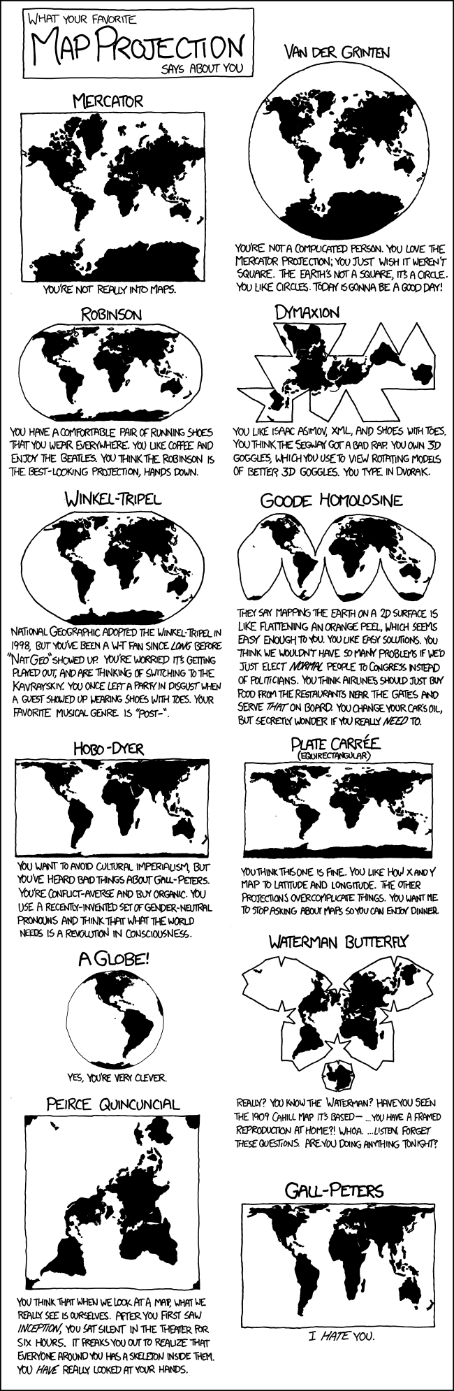
Weird projections
- Often made as compromises between types of distortion
- Like the Waterman Butterfly


![]()

 Left: circles of equal area on globe. Right: same circles on Mercator projection.

 Top: True-color satellite image of Earth in equirectangular projection.
Bottom: Equirectangular projection with Tissot’s indicatrix.

Top: Nautical Chart of Lake Superior in Mercator projection. Bottom: Mercator projection.


UTM
Universal Transverse Mercator (UTM)
- a projection and accompanying projected coordinate system
- Divided into 60 narrow zones
- Does not cover polar regions
- Large north-south extent with low distortion


Image Source: wikimedia
- Open QGIS
- Use QuickMapServices to add a global Satellite coverage layer.
- In the drop down menus, go to Project –> Preferences then select the CRS tab on the left
- In the filter box type “26910”
- Under Predefined Coordinate Reference Systems select NAD83 / UTM zone 10N
- Click Apply and OK
State Plan System
Each State Plane Coordinate System zone uses a map projection based on its geographic orientation.
e.g.
- Transverse Mercator Projection
- Lambert Conformal Conic Projection
- Hotine Oblique Mercator Projection


- Reproject the global satellite image from the last slide to EPSG:2227 (California zone 3)
- Scroll to zoom in on South Africa. What do you notice?
Levels of Measurement
- Nominal - Names or identifiers of objects
- Ordinal - Ranked categories based on a measure
- Ratio - have a 0 value that indicates absence of the quantity of interest
- e.g. Mass, distance, Temperature in Kelvins
- Interval - have a regular scale, but not a meaningful 0 value
- e.g. Date, temperature in C or F
Ratio - Multiplication makes sense, e.g. 200 K is twice as hot as 100 K \[ 2 \times 100 \mathrm{K} = 200 \mathrm{K} \]
Interval - Multiplication does not make sense, e.g. 200°C is not twice as hot as 100°C \[ 2 \times 100°\mathrm{C} \neq 200°\mathrm{C} \]

Image Source: wikimedia
Geospatial Data Types: Vector vs. Raster

Vector Data
- Can be described by points, lines, polygons
- Ex: roads, rivers, train tracks, hiking trails, sidewalks, building footprints, county boundaries
- NOT images, do NOT contain any pixels
- The kind of data we’ve been working with so far

- Stored as tabular data files with geographic metadata
- Points, lines, and polygons represent the spatial features
- Topology describes the connectivity, area definition, and contiguity of interrelated points, lines, and polygon

Points
- Zero-dimensional objects containing a single coordinate pair.
- Ex: Lat/Lon coordinates denoting a city, building, address, etc
- X,Y coordinates on a cartesian plane
Lines
- One-dimensional objects composed of multiple, explicitly connected points.
- Lines have the property of length.
- Also called an “arc.”
Polygons
- Two-dimensional features created by multiple lines to create a “closed” feature.
- First point on the first line segment is the same as the last point on the last line.
- Can represent city boundaries, buildings, lakes, soils, etc.
- Have the properties of area and perimeter.
Structuring Vector Data
- There are several ways to define relationships between vector data:
Feature based: The “Spaghetti Model”
- Each feature is a long string of coordinates
- No relationships between features
Structured: The “Topological Model”
- Enforced relationships between features


Raster Data
- Derived from a grid-based system of contiguous cells containing specific attribute information.
- The spatial resolution of a raster dataset represents a measure of the precision or detail of the displayed information.
- Widely used by technologies such as digital images and LCD monitors.

- Images, stacks of images (satellite / drone image)
- Raster (latin) means “screen”!
- Grids of numbers
- Things with pixels!
- If it’s pixelated:
- It’s a raster
- If it’s a photo:
- It’s a raster
- If it’s a digital image
- It’s a raster!

- The spatial resolution of a raster dataset represents a measure of the precision or detail of the displayed information.
- AKA pixel size
- Ex: 1mm, 1cm, or 1m
- So when you hear that a camera has N megapixels - this just means it has many millions of pixels

Spatial Resolution
The spatial resolution of a raster dataset represents a measure of the accuracy or detail of the displayed information.

The spatial resolution of a raster dataset represents a measure of the accuracy or detail of the displayed information.

Spectral Resolution


You should see something like this when it first opens:

To register, click the “Login” button at the top of the left panel
Follow the steps to register, confirm your email, and then go back to the main page.
Look at the Garnet Fire on CalFire inciweb.
- In Copernicus Browser (in visualize mode), paste the lat, lon into the search, hit enter
- Change the date to 2025-09-07
- Adjust image so the fire is in view

- Lets try a different visualization
- Copernicus offers a SWIR based composite visualization that is quite good for burn detection.


Step One - Registering for GEE
- To connect your Google account, go to https://code.earthengine.google.com/
- Once you’ve logged in, you should see something like this:

- We want to register a new project
- Name your project something useful, then hit create
- Next, we want to register the project for non-commercial use

This will take you to a form where you can confirm your eligibility. Here’s an example of how to fill it out:


These are the main panels to be aware of:

Step Two - Editing and Running a Script
- In the scripts panel, select New > File and name it something useful
- You should see it show up under the Owner dropdown:

- Click on the file to open it, and then move to the Code Editor. It should be blank to start.
- Let’s try running some code! In the editor window, type the following command:

- Then hit run. Look at the console - what do you see?
Next, we’re going to explore some spatial data.
- In the search bar at the top of page, type in “California Polytechnic State University”
- Click on the search result, and the map view should update accordingly
Add a marker to the map by clicking this icon:

Place the point somewhere in the middle of campus:

- At the top of the code editor, you should now see a new var called “geometry”, which gives us the coordinates of our point

- We can now reference the point in new lines of code, like we did with “largeCities”
- To add in other data layers, let’s look in the Earth Engine Data Catalog
- Using the search bar, find the Sentinel-2 Dataset and click on the Level-1C option
- Scroll down to the “Explore with Earth Engine” section, and copy the JavaScript code
- Go back to the code editor, and paste the code onto a new line
Before we run it, let’s make a few changes to the code.
- First, let’s change these dates to be more recent:

- Pick a month in 2025, and set the dates to be the first and end of the month
- Next, let’s change the center point of the map to the point we dropped earlier:

- Replace the entire line with the following code:
- Alternatively, you can just replace the first two numbers with the coordinate values saved to “geometry”
Hit run, and watch what happens in the map viewer! It may take a second for the layer to load.
We can do the same operation we just did through the plugin:

Events


Buffer


- Open QGIS and open the ‘sprStreams.geojson’
- Vector –> Geoprocessing tools –> Buffer
Notice the Units! Buffering in degrees makes no sense. Reproject it first! What is a good projection?

Dissolve

- In QGIS open
sprSoil.geojson - Change symbology to categorical by “SOILNAME”
- Vector –> Geoprocessing tools –> Dissolve
- Use “HYDROGRPOUP” as dissolve field
Clip
- Vector –> Geoprocessing tools –> Clip
- Clip the sprSoil by the streams buffer.
![]()

Spatial overlays
- Intersect soils with bufffer, look at attributes
- Intersect buffer with soils, look at attributes

Union

Symmetric Difference
- Try it with buffer and soils

Joins
Tabular joins join layers by matching a common column name (e.g., parcel_id or GEOID)

Spatial joins transfer attributes based on how features relate in space (intersects, within, nearest)
