Xarray

Working with Spatio-temporal Data

In this tutorial we will be looking at sea surface temperatures using Community Earth System Model 2 (CESM2) data. This tutorial borrows heavily from this tutorial by Computational Tools in Climate Science. That tutorial has much more information about climatology, the focus here is using Xarray for data cubes.

This is gridded climate data given in lat, lon coordinates. In the rioXarray tutorials we will learn to deal with projections etc…

First import libraries and download dataset.

import matplotlib.pyplot as plt
import numpy as np
import xarray as xr
from pythia_datasets import DATASETS
import matplotlib.pyplot as plt


filepath = DATASETS.fetch('CESM2_sst_data.nc')

Open the dataset and inspect. It is an Xarray Dataset. It has coordinates lat, lon, and time. It has corresponding indices It has spatial and time coordinates, hence we call it a spatio-temporal dataset.

ds = xr.open_dataset(filepath)
ds

/home/michael/miniconda3/envs/geo3/lib/python3.12/site-packages/xarray/conventions.py:204: SerializationWarning: variable 'tos' has multiple fill values {np.float32(1e+20), np.float64(1e+20)} defined, decoding all values to NaN.
  var = coder.decode(var, name=name)

You can subset the data along an axis with slicing (here we explicitly create a slice object)

ds.sel(
    time=slice('2004-01-01', '2004-12-31')
)

Check out the attributes (you can click the drop down arrows). Notice the units are degrees C. If you wanted the temperature in Kelvins you can change them very much as you would change a column in Pandas.

ds.tos + 273.15

Boom Kelvins!

Note

Do you notice all of those NaNs? This is sea surface temperature, so where there is land, there is no data.

Aggregations

A common thing to do in performing various types of analysis is to apply aggregations such as .sum(), .mean(), .median(), .min(), or .max(). These methods can be used to reduce data to provide insights into the nature of a large dataset. For example, one might want to calculate the minimum temperature for each cell (temporal minimum).

global_min = ds.tos.min(dim='time')
global_min

Pay attention to the dimensions of the above output. We have collapsed the time dimension using the .min() method, so we are left with a 2D grid of lat and lon.

fig, ax  = plt.subplots();
title = f'Minimum annual SST {ds.time.min().item().year} - {ds.time.max().item().year}'
global_min.plot(cmap='inferno', ax=ax, cbar_kwargs={'label': 'degrees C'});
ax.set_title(title );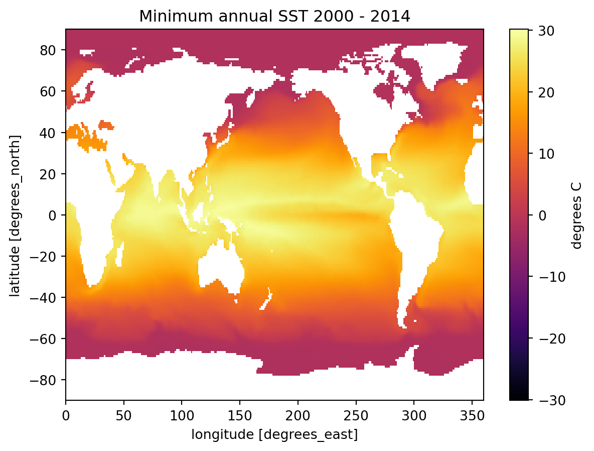

We could also aggregate spatially, for instance we could find the mean the sea surface temperature across the entire grid at eac time step, leaving us with a 1D timeseries of mean temperatures.

t_mean = ds.tos.mean(dim=["lat", "lon"])
t_mean

fig, ax  = plt.subplots();
t_mean.plot()

title = f'Global Mean SST {ds.time.min().item().year} - {ds.time.max().item().year}'
ax.set_title(title);
ax.set_ylabel('degrees C');
ax.set_xlabel('Year');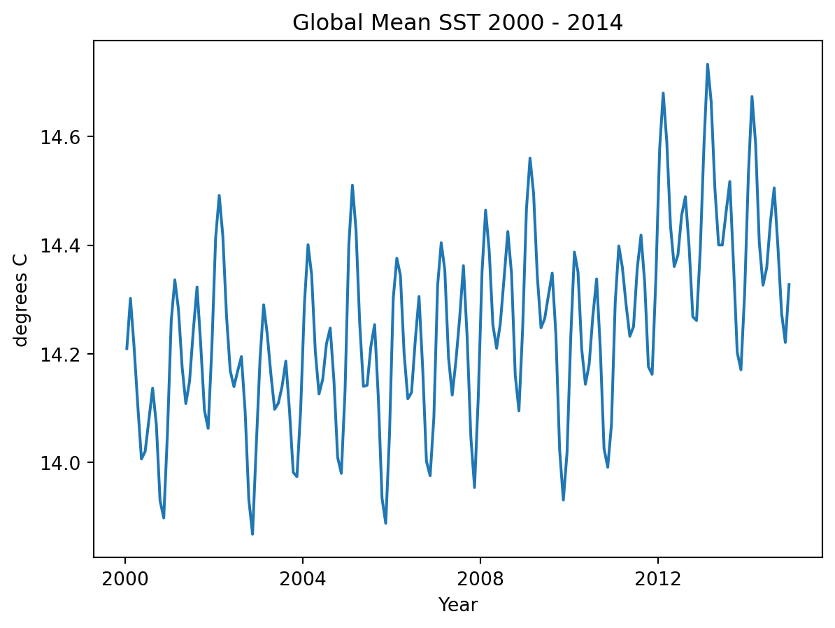

Exercise

Now that you know how to slice and aggregate, find and plot a map of maximum SST for the year 2005.

GroupBy: Split, Apply, Combine

Often it is useful to aggregate conditionally on some coordinate labels or groups.

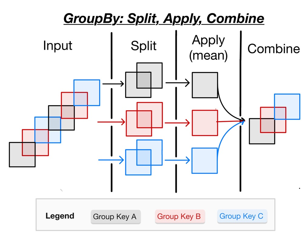
Here we will use a split-apply-combine workflow to remove seasonal cycles from the data.

Here is the splitting alone using .groupby

ds.tos.groupby(ds.time.dt.month)

<DataArrayGroupBy, grouped over 1 grouper(s), 12 groups in total:
    'month': 12/12 groups present with labels 1, 2, 3, 4, 5, 6, 7, 8, 9, 10, 11, 12>

grouped_mean = ds.tos.groupby(ds.time.dt.month).mean()
grouped_mean

For every spatial coordinate (gridded cell center), we now have a monthly mean SST for the time period. So lets look a monthly mean off the coast of San Luis Obispo.

fig, ax  = plt.subplots();
grouped_mean.sel(lon=238, lat=35.2289, method='nearest').plot();
ax.set_title('Monthly mean SST off the coast of SLO');
ax.set_xlabel('Month');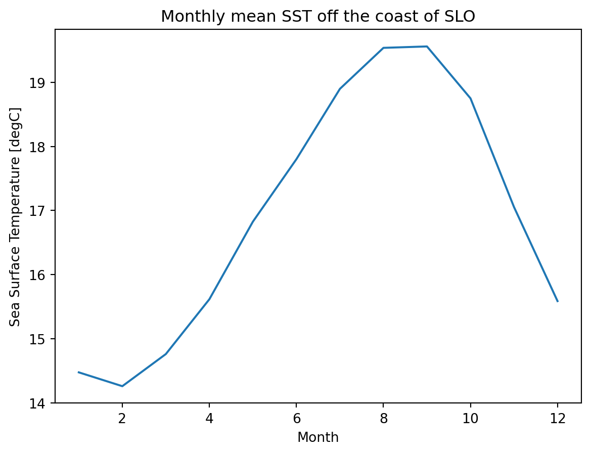

Question???

What are these trailing semicolons all about? Python does not typically end lines with a semicolon. Experiment with the above code block with and without the semicolons.

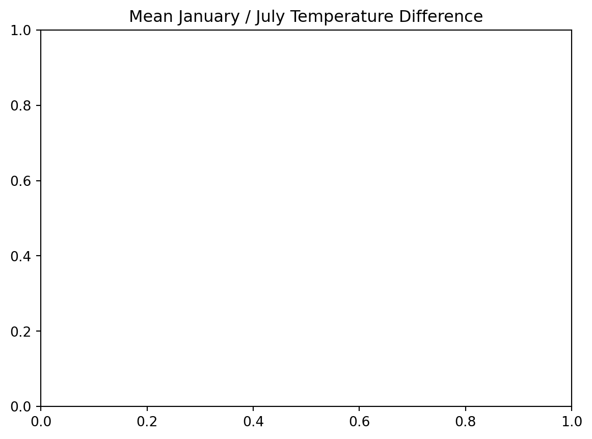
fig, ax  = plt.subplots();
(grouped_mean.sel(month=1) - grouped_mean.sel(month=7)).plot(ax=ax, robust=True)
ax.set_title('Mean January / July Temperature Difference');